DL M1: Linear Classifiers and Gradient Descent
Module 1 of CS 7643 - Deep Learning @ Georgia Tech.
Machine Learning: An Overview
What is Machine Learning?
Machine Learning is the study of computer algorithms that improve performance on some set of tasks based on experience, where experience typically comes in the form of data.
A computer program is said to learn from experience E with respect to some class of tasks T and performance measure P, if its performance at tasks in T, as measured by P, improves with E.
- Tom Mitchell (Machine Learning, 1997)
How is machine learning different from programming?
- Programming uses some programming language to define a series of instructions which accomplish some task.
- Machine learning uses some programming language to define a learning algorithm, which outputs a model to perform some task.
- Instead of writing code to directly accomplish the task, we write code to produce a model which accomplishes the task for us.
- Machine learning is particularly useful in situations where it is difficult to design an algorithm to directly perform the task.
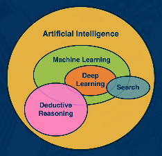
Machine learning is a subset of Artificial Intelligence - the field concerned with understanding and constructing intelligent entities to act rationally in a wide variety of novel situations.
Example applications of machine learning include…
- Computer Vision: enables machines to process, analyze, and interpret images.
- Natural Language Processing: helps machines to understand and communicate using human language.
- Time Series Prediction: generate an informed forecast based on a series of observations.
- Reinforcement Learning: teaches autonomous agents to make decisions by interacting with their environment.
There are three major subfields of machine learning (briefly summarized as follows):
- Supervised Learning: function approximation.
- Unsupervised Learning: data description.
- Reinforcement Learning: decision making.
Supervised Learning and Parametric Models
Supervised Learning is the division of machine learning concerned with function approximation. Given some labeled data - where labeled implies we have some designated output of interest $Y$ - supervised learning trains a model to predict the output $y$ based on input data $X$. \(f : X \rightarrow Y\) Classification refers to the set of supervised learning problems where the output is discrete (finite). Conversely, regression indicates the output is continuous.
The supervised learning model itself takes one of two major forms:
- Non-Parametric: does not explicitly specify a model for the function $f : X \rightarrow Y$, nor make any strong assumptions regarding the structure of the data.
- ex: K-nearest neighbors
- Parametric: explicitly models the function $f : X \rightarrow Y$ using a fixed number of learnable parameters. Assumes certain properties of the data (ex: distribution).
- ex: Linear regression
Linear Classifier
One type of parametric model is the linear model, which assumes the relationship between input features $x_d$ and output $z$ is linear (i.e., output is a weighted sum of the inputs). \(z = w_1x_1 + \dots + w_dx_d + b = Xw + b\) A Linear Classifier uses the linear model to perform classification. For example, binary logistic regression normalizes the output of a linear model $z$ to a valid probability distribution over two classes $y$.
\[y = \sigma(z); ~~ \text{Sigmoid}: \sigma(z) = \frac{1}{1 + e^{-z}}\]In the case of binary classification, we have a single logit (unnormalized score $z$) corresponding to our positive class. This enables us to use the sigmoid function to convert our score to a probability for the positive class.
But what if we have more than two classes? Multinomial logistic regression is a similar approach which calculates the probability corresponding to each class. As part of multinomial logistic regression, we have a different set of weights corresponding to each class.
\[W = \begin{bmatrix} w_{(1,1)} & \ldots & w_{(1, d)} \\ \vdots & \ddots & \vdots \\ w_{(c, 1)} & \ldots & w_{(c, d)} \end{bmatrix}; ~~~~ z = \begin{bmatrix} z_1 & \ldots & z_c \end{bmatrix} = XW^T + b\]Our logit vector is transformed to a valid probability distribution using the softmax function.
\[\text{Softmax}(z_i) = \frac{e^{z_i}}{\Sigma_j e^{z_j}}\]Note that sigmoid is actually a generalization of softmax where we have two classes, and assume the score for the negative class is 0.
Performance Metrics
Parametric supervised learning approaches (such as the linear classifier) require some key components to identify the optimal set of parameters:
- Loss Function: evaluates the current model (including set of parameters).
- Optimization Algorithm: strategy for updating parameter values to decrease loss.
With these components in mind, note that parametric model training is an optimization procedure - we are interested in identifying the best set of parameter values to minimize loss. So what is our loss function? It depends on our problem type.
- Regression: mean squared error measures the average difference between our predictions $\hat{y}$ and true output $y$.
- Classification: cross entropy measures the difference between our predicted probability distribution over classes $\hat{y}$ and our true probability distribution over classes $y$.
- $\Pr(y_i = c)$ is the probability of the true output being the class of interest $c$. Note that $\Pr(y_i = c)$ is always 1 for the correct class and 0 for all other classes.
- $\Pr(\hat{y_i} = c)$ is the probability of the predicted output being the class of interest $c$. Our model outputs an estimated probability distribution over all classes. We only use the estimate for the correct class $c$ as part of the loss function.
We often add a regularization term to the loss function to constrain our optimization problem. For example, L1 and L2 penalty terms may be added to the loss function to limit the size of our parameter values (and thus mitigate high variance = overfitting).
- L1 Loss $|W|$: sum of absolute values of parameters.
- L2 Loss $|W|^2$: sum of squared values of parameters.
Optimization
Given a model and loss function, finding the best set of parameters is an optimization problem. In machine learning, we typically use gradient-based optimization to update parameter values in a data-driven manner.
Gradient Descent is a specific algorithm which iteratively updates parameter values using the derivative of the function with respect to each parameter. The direction of steepest ascent for a function is denoted by the gradient; therefore, steepest descent is represented by the negative gradient.
\[f'(a) = \lim_{h\rightarrow0} \frac{f(a + h) - f(a)}{h}\]In machine learning, we are interested in knowing how the loss function changes as weights are varied. Therefore, we will compute the partial derivative of the loss function with respect to each parameter in our model to perform updates.
Gradient descent involves two main steps:
- Calculate the Gradient - derivative of loss function with respect to each model parameter.
- Update model parameters by taking a step in the direction of the negative gradient.
- step size is controlled via the learning rate hyperparameter.
Standard gradient descent involves computing the gradient over the entire dataset at each iteration (called the batch). However, this can be computationally expensive. Instead, stochastic gradient descent (SGD) is a variant which uses a mini-batch - sub-sample of the training set - to estimate the gradient at each step.
Deep Learning
Deep Learning is the application of deep differentiable networks - typically in the form of neural networks with 2 or more hidden layers - to machine learning problems. But how is this any different from standard machine learning? Deep learning has a few key characters setting it apart from other machine learning methods.
Hierarchical Compositionality
Deep learning involves Hierarchical Composition via a series of linear / non-linear transformations represented via layers. The neural architecture of a deep learning model refers to its arrangement and type of layers. Neural architecture can be varied to match the task at hand, learning intermediate representations at earlier layers of the model informative for subsequence layers.
Note that a deep learning model is simply a composition of functions.
\[f(x) = g_1(g_2(\ldots(g_n(x))))\]As long as the function is differentiable (making it compatible with gradient-based optimization procedures), it can be included as part of a deep learning model.
End-to-End Learning
As opposed to classical machine learning algorithms, deep learning is an End-to-End Learning process which learns representations of the input useful in accomplishing the task.
Classical machine learning algorithms require hand-designed feature engineering, which typically involves trial-and-error / exploration. Conversely, the hierarchical nature of deep learning algorithms enables it to perform feature extraction by learning intermediate hidden states as transformations of the original input. In this way, feature extraction is bundled into the network itself in an automated and optimization-based fashion.
Distributed Representations
Finally, deep learning uses a Distributed Representation via connections across a large number of nodes, enabling it to learn to represent complicated structures. Since each node represents a different aspect of the data, we can combine them in complex ways to generate a wide range of outputs.
Mathematical Considerations
Linear Algebra
Recall that a vector-valued linear model with $o$ outputs is structured as follows:
\[z = \begin{bmatrix} z_1 & \ldots & z_o \end{bmatrix} = XW^T + b\]Let’s take a closer look at the dimensions of each term and see why this mathematical representation makes sense.
$W$ is a matrix with each row corresponding to the weights for a particular output; we will represent our number of outputs as $o$. Each row contains a parameter for each of our input features in $X$, which we will represent as $p$.
\[W \sim (o, p); ~~ W = \begin{bmatrix} w_{(1,1)} & \ldots & w_{(1, p)} \\ \vdots & \ddots & \vdots \\ w_{(o, 1)} & \ldots & w_{(o, p)} \end{bmatrix}\]Our input $X$ is a matrix consisting of $n$ rows corresponding to each instance (instance = single entity), and $p$ columns corresponding to each feature (feature = variable in our input data).
\[X ~ (n, p); ~~ X = \begin{bmatrix} x_{(1,1)} & \ldots & x_{(1, p)} \\ \vdots & \ddots & \vdots \\ x_{(n, 1)} & \ldots & x_{(n, p)} \end{bmatrix}\]As part of the linear model, we are interested in taking the dot product between each instance $x_n$ and each weight vector $w_o$. This will produce a vector of output values $z_o$ for each instance. Applied over many different instances, this will produce a matrix with $n$ rows corresponding to each instance and $o$ columns corresponding to each output.
\[XW^{T} \sim (n, o)\]Finally, we add some bias term to each output score to shift our linear combination as desired.
\[b \sim (1, o); ~~~ XW^T + b \sim (n, o)\]Derivative Sizes
Recall that we use gradient descent to optimize our parameter values in the weight matrix with respect to some loss function. A gradient-based optimization procedure uses the partial derivatives of our loss function with respect to each input to iteratively update parameter values, stepping towards some minimum for loss. But how many partial derivatives will we have? It turns out there are two primary cases.
When we have a scalar-valued multivariable function, we obtain the gradient - a vector of partial derivatives for each parameter $w$ with respect to the output variable $y$. More generally, the gradient represents the partial derivative of a scalar with respect to a vector.
\[y = Xw + b; ~~~~~~~~~~ y \in \mathbb{R}^{(1 \times n)}, ~~ w \in \mathbb{R}^{(1 \times p)}, ~~ X \in \mathbb{R}^{(n \times p)}\] \[\frac{\partial{y}}{\partial{w}} = \begin{bmatrix} \frac{\partial{y}}{\partial{w_1}} & \ldots & \frac{\partial{y}}{\partial{w_p}} \end{bmatrix}\]In the case of a vector-valued multivariable function, we have the Jacobian - a matrix of partial derivatives for each parameter $w$ with respect to each output $y \in Y$. More generally, the Jacobian represents the partial derivative of a vector with respect to a vector.
\[Y = XW^T + b; ~~~~~~~~~~ y \in \mathbb{R}^{(n \times o)}, ~~ w \in \mathbb{R}^{(o \times p)}, ~~ X \in \mathbb{R}^{(n \times p)}\] \[\frac{\partial{Y}}{\partial{W}} = \begin{bmatrix} \frac{\partial{y_1}}{\partial{w_1}} & \ldots & \frac{\partial{y_1}}{\partial{w_p}} \\ \vdots & \ddots & \vdots \\ \frac{\partial{y_o}}{\partial{w_1}} & \ldots & \frac{\partial{y_o}}{\partial{w_p}} \end{bmatrix}\]Things get more complicated when our input dimensionality increases. For example, we typically work with higher-rank Tensors - multi-dimensional arrays with rank $n$ - for inputs such as image data. We will examine this math in future lessons.
(all images obtained from Georgia Tech DL course materials)