DL M10: Language Modeling (Meta)
Module 10 of CS 7643 - Deep Learning @ Georgia Tech.
Introduction
A Language Model estimates the probability distribution over sequences of words.
\[\Pr(s) = \Pr(w_1, \ldots, w_n)\]Note that more generally, we are interested in estimating the probability distribution for the next word in a sequence given the history of words that have occurred before it. We can expand the above equation using the product rule of probability.
\[\Pr(s) = \prod_i \Pr(w_i | w_{i-1}, \ldots, w_1)\]This sequential construction demonstrates how language models are capable of generating words. Once we’ve estimated the probability distribution over all possible values of $w_i$, we can take the argmax of our distribution to predict the next word in a sequence.
Conditional language modeling is a slight variation on language modeling which incorporates some additional constraint into the probability calculation.
\[\Pr(s|c) = \prod_i \Pr(w_i | c, w_{i-1}, \ldots, w_1)\]The condition $c$ is intentionally vague so that it may generalize to many possible scenarios; for example, $c$ may be a topic in topic-aware language modeling, a long document in the case of text summarization, a source language in the case of machine translation, and so on.
RNNs
A Recurrent Neural Network (RNN) is a class of neural network architectures dedicated to modeling sequential data. RNNs make use of recurrence to utilize information from previous time steps in the prediction for the current time step.
Traditional multi-layer perceptrons (MLPs) are not a great fit for sequence data. MLPs have strict requirements for input dimensionality (i.e., fixed number of features), but sequence data is variable-length. Since RNNs process sequence data in an iterative manner, they are able to process variable-length sequences with no issue. Furthermore, MLPs have no inherent temporal structure, whereas RNNs introduce an architectural bias to account for temporality.
Forward Propagation
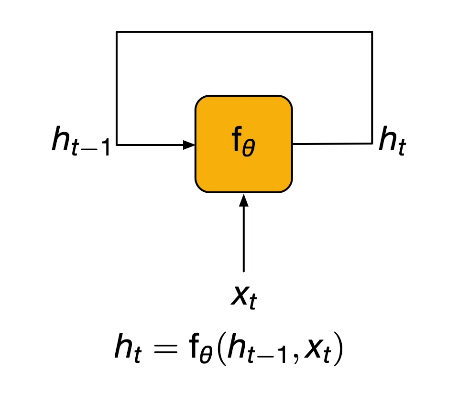
At every time step, a recurrent unit receives some input $x_t$ and the Hidden State from the previous time step $h_{t-1}$. The input is then used to generate the hidden state for the current time step $h_t$.
In the context of RNNs, unrolling refers to expanding the computation graph along the time axis. This provides a more linear view of the recurrent computation.
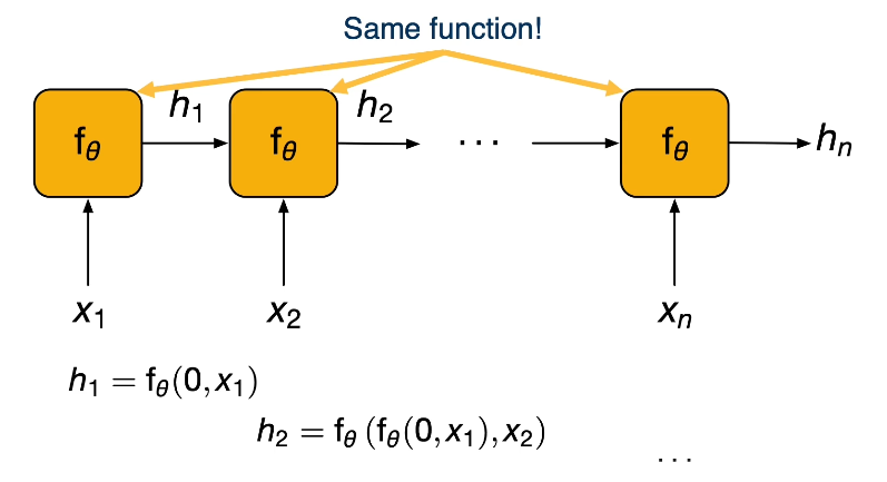
Notice that the same weight matrix (represented as $\theta$ above) is used to transform our input, regardless of time step. This implies that RNNs make use of parameter sharing.
The Elman RNN is the simplest (vanilla / default) example of an RNN. The recurrent layer is a combination of a linear transformation of the input $x_t$, with another linear transformation applied to the hidden state $h_t$. The result is then passed through a non-linear activation function to yield the final output hidden state.
\[h_t = \sigma(Ux_t + Vh_{t-1} + b_h)\]Once we have our hidden state, we can transform to output dimensionality to get our final predicted probability distribution over outputs (which are words in our vocabulary in language modeling).
\[o_t = \sigma(Wh_t + b_o)\]Backpropagation
In the case of RNNs, Backpropagation applies similarly to any other neural network once we unroll the computation graph. The combination of backpropagation and unrolling through time is sometimes called backpropagation through time. Note that the unrolling operation scales to the number of time steps in our history; for words occurring later in the sequence, we will have a longer chain. This is the primary reason why RNNs have issues with vanishing / exploding gradients.
\[x_t = \sigma(w_{\theta}x_{t-1}); ~~~~~\frac{\partial x_t}{\partial x_0} \propto w^t_{\theta}\]- $|w_{\theta}| > 1$: exploding gradient
- $|w_{\theta}| < 1$: vanishing gradient
LSTMs
Long Short-Term Memory (LSTM) architecture aims to relieve the problem of vanishing / exploding gradients. LSTMs use a series of gates to update cell state, which preserves information in a more complex (and thus more representative) way across time steps.
- Forget Gate $f$: decides which information to remove from previous cell state.
- Input Gate $i$: decides which information to incorporate from input into cell state.
- Output Gate $o$: decides how much of resulting cell state passes to next layer.
Language Modeling
Given an RNN and body of text, how can we actually train a machine learning model to generate text?
Text Representation
As you might expect, text can’t be used in its raw form as input to machine learning models. We can represent each word as a one-hot vector, where each word in our vocabulary has a unique index called a token. This means a sequence of text can be converted to a sequence of one-hot vectors. Given vocabulary dimensionality of $|V|$ and sequence length of $m$, each sequence will be of shape $(n \times |V|)$.
In addition to the unique words in our language, we may also add other special tokens to our vocabulary:
- $<$sos$>$: start-of-sequence
- $<$eos$>$: end-of-sequence
- $<$unk$>$: unknown
- $<$pad$>$: blank token which should not be considered
Inference
During inference, we use a trained model to perform predictions on data. This works by feeding each token in the sequence to the model. Recall that any RNN outputs two values: the hidden state from some intermediate portion of the network, and the actual prediction for the time step. Intermediate predictions can be discarded until reaching the point of our sequence where we’d like to actually generate output.
Training
During RNN training, we use teacher forcing to feed the network correct intermediate inputs at each time step. This ensures the model learns in a more rapid manner, considering if it used its own intermediate predictions, it might have trouble identifying the real patterns in the data.
Evaluation
Cross Entropy (CE) is typically used as the loss function for language model tasks such as text generation. Cross entropy calculates the expected number of bits required to represent an event drawn from the reference distribution $\Pr^*$ when using a coding scheme $\Pr$. Put more casually, cross entropy is a method to measure the difference between two probability distributions.
\[H(\Pr^*, \Pr) = - \Sigma_{x\in X} \Pr^*(x) \log \Pr(x)\]Per-word cross entropy is the application of cross entropy to a sequence of words. Given that the $i$-th word of the sequence is known, we estimate the true probability of its occurrence as $\Pr^*(w_i) = 1$.
\[H = -\frac{1}{N} \Sigma_{i \in N} \log \Pr(w_i | w_{i-1}, \ldots)\]Perplexity is another evaluation metric, which represents the level of confusion a model may have when generating a prediction. It is calculated as the geometric mean of the inverse probability of a sequence of words.
\[\text{Perplexity(s)} = \prod_i \sqrt[\leftroot{10} \uproot{5} n]{\frac{1}{\Pr(w_i|w_{i-1}, \ldots)}}\]To better visualize perplexity, note that the perplexity of a discrete uniform distribution over $k$ events is $k$. For example, the perplexity of flipping a fair coin is 2. If we have a stronger probability distribution favoring certain categories, our perplexity will be smaller.
Masked Language Modeling
We can use Masks in conjunction with language modeling to learn effective contextual representations of these words (and thus better approximate language generation).
- Convert a sequence of words to a sequence of tokens.
- Replace (perhaps randomly) certain tokens with a special token to indicate the mask.
- Construct a model to predict the masked tokens.
Masked language modeling is often applied as a pre-training task to boost language model performance relative to a particular target task. This is because the concept of predicting masked words helps the model to learn about the structure of language, which applies to pretty much any language modeling task.
Knowledge Distillation
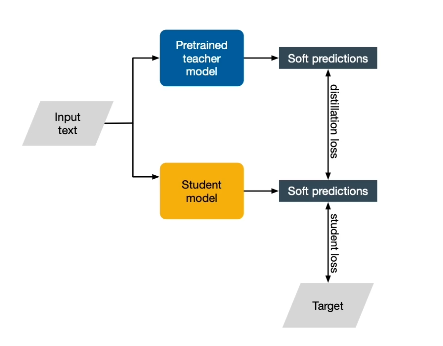
Consider the typical method for training an NLP model. We have some input text, which is used to train a model and generate predictions, which can then be evaluated relative to some ground truth target via a loss function.
Knowledge Distillation works slightly differently. It turns out that the best NLP models tend to be massive foundation models, which are pre-trained on a huge amount of data and have many parameters. If inference with the large model is computationally expensive, we can train some student model with a smaller number of parameters based on the predictions of the larger model.
(all images obtained from Georgia Tech DL course materials)