DL M11: Neural Attention Models (Meta)

Introduction

Attention is a neural mechanism that weights elements of a set for use by the network in the current computation. It enables a network to dynamically attend to different portions of the input depending on relevance to the current information being passed through the network.

Attention is a powerful technique used across subfields of deep learning, including computer vision and natural language processing.

Softmax

Recall that the Softmax function converts a set of numbers into a probability distribution.

\[\text{Softmax}(\begin{Bmatrix}x_1, \ldots, x_n \end{Bmatrix}) = \begin{Bmatrix} \frac{e^{x_1}}{\Sigma_i e^{x_i}}, \ldots, \frac{e^{x_n}}{\Sigma_i e^{x_i}} \end{Bmatrix}\]

Sigmoid vs. Softmax

Softmax is a generalization of the sigmoid function, which is used in the case of binary classification. As part of binary classification, we have two scores: the score obtained from our classification model for the positive class $s_+$, and the implicit score of 0 for the negative class. Consider the case of $s_+ = 6$.

\[\text{Softmax}(\begin{Bmatrix} 0, 6 \end{Bmatrix}) = \begin{Bmatrix} \frac{e^0}{e^0 + e^6}, \frac{e^6}{e^0 + e^6} \end{Bmatrix} = \begin{Bmatrix} 0.0025, 0.9975 \end{Bmatrix}\] \[\sigma(6) = \frac{1}{1 + e^{-6}} = 0.9975\]

We can also show that the sigmoid function is mathematically equivalent to softmax in the case of a single positive class score, and negative class score of 0.

\[\text{Softmax}(s_+) = \frac{e^{s_+}}{e^{s_+} + e^0} = \frac{\frac{e^{s_+}}{e^{s_+}}}{\frac{e^{s_+}}{e^{s_+}} + \frac{1}{e^{s_+}}} = \frac{1}{1 + e^{-s_+}}\]

Softmax Characteristics

Greater input scores result in a greater difference in the resulting probability distribution. For example, the probability corresponding to the argmax class will be higher when all input scores are doubled.

The most important property of softmax is that it is differentiable. This is why the function is called “soft”max, since it is a software version of argmax.

By generating a probability distribution over the input elements, softmax can be used to randomly sample from the inputs. This is particularly useful in the case of attention.

Attention

Attention refers to the process of weighting a set of vectors to be used in combination with some input for a prediction, within the context of a neural network. Mathematically, attention calculates a distribution over its inputs depending on similarity between some query vector, a set of keys, and a set of values.

• Query $q$: internal hidden state; input to the attention layer.
• Keys $K$: set of embeddings labeling each element of the set.
  • Similarity is calculated between each query : key combination. $s = \text{Softmax}(\frac{q \cdot K^T}{|q| \times |K|})$
• Values $V$: content or information associated with each key.
  • Weighted sum is calculated using similarity scores and keys. $a = s \cdot V$

In the case of self-attention, the $K$ and $V$ are calculated within the same attention layer as $q$. Cross-attention pulls $K$ and $V$ from another network or layer.

Differentiable Motivation

In the case of attention, we want to identify the most similar vector to an input (query) vector. Given our set of key vectors $\begin{Bmatrix} k_1, \ldots, k_n \end{Bmatrix}$ and a query vector $q$, we can select the most similar vector by maximizing the dot product (recall that the dot product is unscaled cosine similarity).

\[\hat{j} = \arg \max_j u_j \cdot q\]

However, since the argmax function is not differentiable, we cannot use it as part a neural network (since we can’t apply backpropagation). Due to its differentiable nature, softmax can be used instead! Attention calculates the similarity scores between each key vector and query, then converts the resulting scores to a probability distribution via softmax.

\[\text{Let} ~ K~ \text{represent the set of vectors}\] \[p = \text{Softmax}(q \cdot K^T)\]

Implementation within Neural Networks

Attention as a neural network layer is a relatively new development (~2013). As mentioned earlier, attention is computed as follows:

1. Calculate the dot product between a set of key vectors and a query vector.
2. Pass the resulting scores through the softmax function.
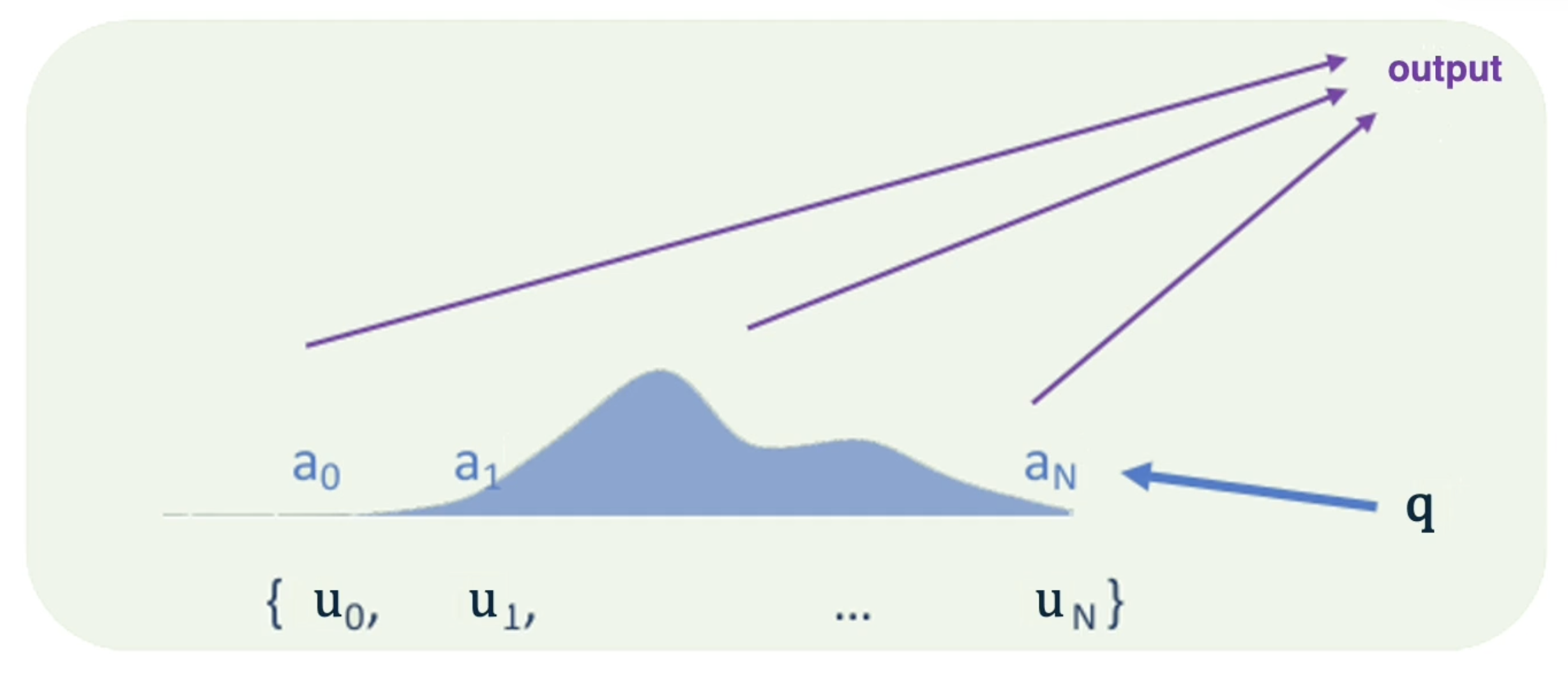
3. Use the resulting probability distribution to perform a weighted sum over value vectors.

Assume that $K = V = \begin{Bmatrix} u_1, \ldots, u_N \end{Bmatrix}$, and that $a$ represents the attention weights.

\[a_j = \frac{e^{u_j \cdot q}}{\Sigma_k e^{u_k \cdot q}}\] \[\text{output} = \Sigma_k a_k u_k\]

There are certain variants of attention commonly used in practice:

• Multi-Layer Attention: chain of attention layers which repeatedly updates the query state.
• Multi-Headed Attention: multiple different attention calculations run in parallel within the same attention layer.

Transformers

A Transformer is a neural network which implements multi-layer attention, and is currently state-of-the-art for most language modeling tasks (as well as other subfields of deep learning). Transformers have the following key components:

1) Self Attention: attention where input to the layer is also considered the set of keys. - $q_i \in K, ~~ K = V$ (lecturer refers to $K = V$ as set of controller states $U$) 2) Multi-Headed Attention: splits attention calculation into multiple heads - subdivisions of the key set - that work in parallel. Each head independently attends to the input, but learns to focus on a different type of information or relationship. 3) Residual Connections: not specific to transformers, but used to help stabilize the gradient when backpropagating through deep neural networks.

We can think of the combination of self-attention and multi-headed attention as an $N ~ \text{x} ~ M$ situation:

• $N$ represents the number of terms within the input. (ex: number of words in input sequence). A context vector is maintained for each term.
• $M$ represents the number of attention heads. Each attention head calculates attention from a different perspective, thus attending to a different aspect of the input.

For each of the $N$ positions, the $M$ context vectors are concatenated and passed through a linear layer. This produces a rich output vector for each of the original $N$ terms, which may then be passed to the next layer of the network.

---

(all images obtained from Georgia Tech DL course materials)