DL M18: Unsupervised and Semi-Supervised Learning

Introduction

We have previously presented machine learning in terms of its three core subdivisions - two of which are…

• Supervised Learning: function approximation for labeled data. $f : X \rightarrow Y$
• Unsupervised Learning: data description for unlabeled data. $f(X)$

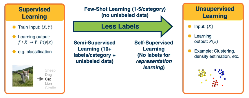
It turns out the distinction between supervised and unsupervised learning isn’t so black-and-white, but rather exists on a spectrum of low-labeled learning.

Traditional unsupervised learning methods also have parallel applications in deep learning:

• Density Estimation: model $\Pr(X)$; similar to Deep Generative Modeling.
• Clustering: compare or group instances; similar to Metric Learning + Deep Clustering.
• Principal Component Analysis: learn lower-dimensional representation; almost all of Deep Learning!

So how can we deal with unlabeled data? Although the approach depends on the task, we may use concepts from unsupervised learning to assist here:

• Semi-Supervised Learning: supervised learning task with a large amount of unlabeled data, and small amount of labeled data.
  • Solution $\rightarrow$ Pseudo-Labeling: train model on labeled data, generate predictions, and assign labels for most confident predictions.
• Few-Shot Learning: supervised learning task with only a handful of labeled observations.
  • Solution $\rightarrow$ Meta-Learning: effectively learns to learn based on small number of SGD steps.
• Self-Supervised Learning: no labeled data.
  • Solution $\rightarrow$ Surrogate Tasks: derive loss functions for alternative tasks, that end up forcing the neural network to learn some good feature representation.

We will consider each of these topics in greater detail below.

Semi-Supervised Learning

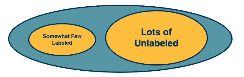
Semi-Supervised Learning refers to the scenario in which we wish to perform a supervised learning task, but have relatively few labeled instances. This often happens in practice since it’s often much cheaper to get large-scale unlabeled datasets.

Can we overcome the small amount of labeled data we have, using the larger amount of unlabeled data? There are several simple ideas which work well in the context of semi-supervised learning:

• Pseudo-Labeling: learn model on labeled data, make predictions on unlabeled data, add as new training data, and repeat.
• Augmentation: used in combination with pseudo-labeling. Given a pseudo-labeled image, create two versions - weakly augmented vs. strongly augmented. Perform model inference on both instances, then minimize cross entropy between pseudo-label for weakly augmented instance and predicted distribution for strongly-augmented instance.

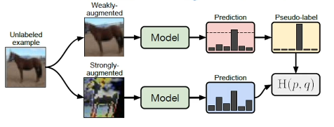
One of the benefits of pseudo-labeling approaches to semi-supervised learning is that these methods can easily be scaled up via larger amounts of unlabeled data. One of the most effective modern pseudo-labeling methods is known as FixMatch.

There are alternative approaches to semi-supervised learning. For example, Label Propagation works by learning feature extractors to cluster cluster data (containing labeled and unlabeled instances). Unlabeled instances are labeled according to similarity to labeled instances.

Few-Shot Learning

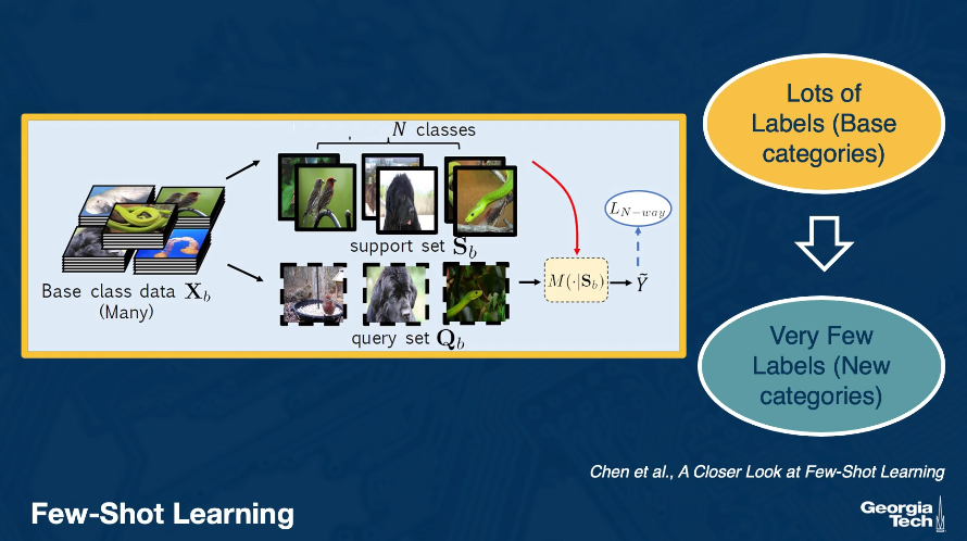
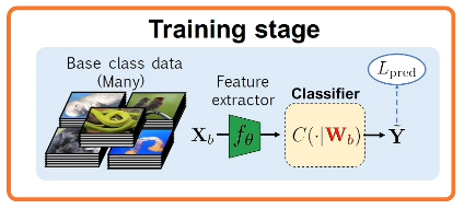
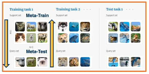
Few-Shot Learning involves a supervised learning task with many labeled instances for base categories, but very few (1-5) labeled instances for previously unobserved specialty categories. We denote our base category data as the support set, and the specialty category data as the query set.

Can we learn an effective representation using the support set, which generalizes to the query set? There are several approaches to few-shot learning:

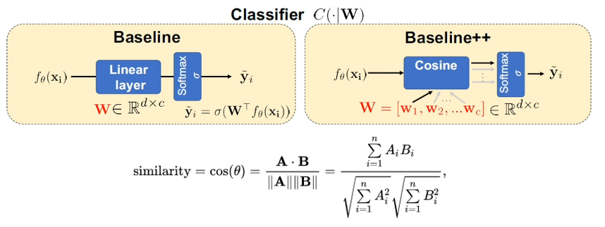
• Fine-Tuning: train classifier on support set, freeze feature extractor, and replace output classifier to be specific to query set. This is a surprisingly effective baseline, even for very few instances!
  • Some research demonstrates that alternative output layer modules (as opposed to fully-connected layers) may be more useful in the few-shot setting. For example, the Cosine Classifier relies on similarity between learned weights and inputs to predict output.

• Meta-Learning: simulate few-shot learning during model training, to better prepare the model to learn relative to unseen categories. Reformulate training data as n-way k-shot tasks with corresponding support and query sets.
  • Can also pre-train features on held-out base classes, then perform meta-learning after.
  • The key idea is that we are parameterizing the learning algorithm itself to increase learning effectiveness, which is desirable given very few training instances for the support set!

Okay, so how do we parameterize the learning algorithm? First, we must define some modeling approach to represent the learning process. For example, a gradient descent meta-learner might learn an optimal parameter initialization and/or update rule. \(\theta_t = \theta_{t-1} - \alpha_t \nabla L(\theta_{t-1})\) This is quite similar to the structure of the cell state mechanism underlying Long Short-Term Memory (LSTM) networks.

\[c_t = f_t \odot c_{t-1} + i_t \odot \tilde{c}_t\]

• $c_t$ represents the model’s parameter space $\theta_t$
• $c_0$ is a learned initialization for the parameters.
• state update $\tilde{c}t$ is the negative gradient $-\nabla(\theta{t-1})$
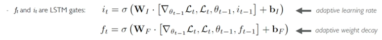
• $f_t$ and $i_t$ are LSTM gates, learned as a function of the gradient and previous gate values. Conceptually…
  • $i_t$ might represent an adaptive learning rate, since it corresponds to $\alpha$ in GD
  • $f_t$ might represent an adaptive weight decay, since it is multiplied with the previous weight set $\theta_{t-1}$

Other competing algorithms learn sub-components of gradient descent, as opposed to using this complicated LSTM-based representation. The general approach - referred to as Model-Agnostic Meta-Learning (MAML) - simply involves backpropagating through gradient descent itself to iteratively improve the model training process.

Self-Supervised Learning

In the case of Unsupervised Learning, we are given unlabeled data $X$ and tasked with investigating its structure. Self-Supervised Learning involves generating labels for a completely unlabeled dataset.

Since we only have unlabeled data, we might start with techniques inspired by unsupervised learning:

• Dimensionality Reduction: learn some lower-dimensional latent representation $Z$ of the input $X$ (via something like an autoencoder). Then, use $Z$ as part of a classifier to predict the outcome.
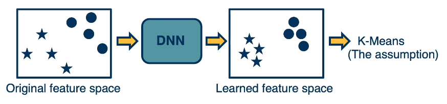
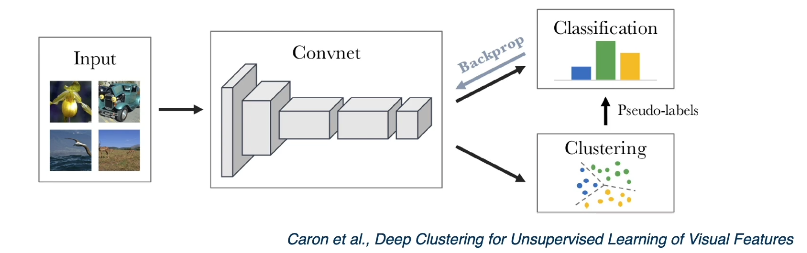
• Clustering: given the assumption that high-density (similar) regions form clusters, learn a feature space that results in distinct clusters.
  • Use resulting clusters as pseudo-labels to drive backpropagation.

Note that in both of the above methods, we actually perform learning relative to an alternative task (as opposed to our primary goal):

• Dimensionality Reduction via Autoencoder $\rightarrow$ alternative task is to minimize reconstruction error, task of interest is to find effective feature representation.
• Clustering with DNN $\rightarrow$ alternative task is to cluster instances, task of interest is to find effective feature representation as part of CNN.

More generally, Surrogate Tasks are alternative objectives used to generate unsupervised feature representations. In the context of image data, example surrogate tasks include jigsaw, rotation, and colorization - these tasks may help us to learn effective features for image-based feature learning.

How do we evaluate the results of training on surrogate tasks?

1. Extract the encoder (feature extractor) portion of the learned network.
2. Perform transfer learning specific to the target task, and score the results.

Overall, there are a large number of surrogate tasks and variations to generate informative features. Two recent methods have been particularly dominant:

• Contrastive Losses: discrimination between positive (augmented but matching) versus negative (non-matching) instances.
• Pseudo-Labeling with Knowledge Distillation.

Augmentation is used across many surrogate tasks, suggesting its effectiveness in producing good representations!

---

(all images obtained from Georgia Tech DL course materials)