DL M2: Neural Networks

Neural Networks: An Overview

A Neural Network is a machine learning model consisting of an interconnected network of nodes, where each node represents some intermediate value within the network. Nodes are stacked within layers, and edges connecting nodes represent some form of computation.

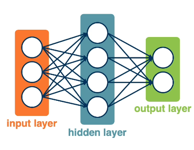
Any layers between the input and output layer are referred to as hidden layers, since their values are not readily available in the final result. Layers can be sequentially arranged to form Deep Neural Networks (DNNs), which are simply neural networks with two or more layers (excluding the input layer).

Mathematically, a neural network is a series of transformations. For example, a simple two-layer neural network can be represented as follows:

\[f(X, W_1, W_2) = g_2(g_1(x)); ~~ g_2(H) = \sigma(HW_2^T + b_2), ~~ g_1(X) = \sigma(XW^T + b_1)\]

We can use any differentiable function as an intermediate layer within a neural network, as to stay compliant with the requirements for gradient-based optimization.

Neural Network View of a Linear Classifier

A simple neural network has a similar structure to a linear classifier.

• linear transformation: weighted sum of inputs and parameters.
• non-linear activation: non-linear function (e.g., sigmoid) is applied to weighted sum.

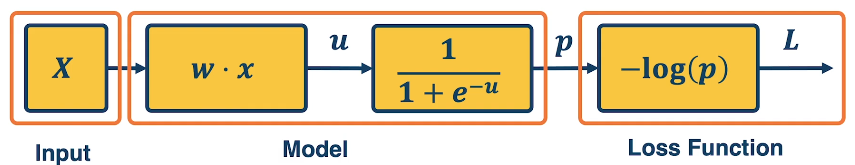
A linear classifier is a particular type of neural network layer in which a certain number of inputs are used to generate a certain number of outputs. Layers that have dense mappings - connections between all possible pairs of input / output nodes - are referred to as Fully-Connected Layers.

Computation Graph

The Computation Graph is a graphical representation of a neural network, illustrating the path of forward propagation through a network. Note that forward propagation is simply the propagation of information forward through a neural network to generate the output.

\[f(x_1, x_2) = \ln(x_1) + x_1x_2 - sin(x_2)\]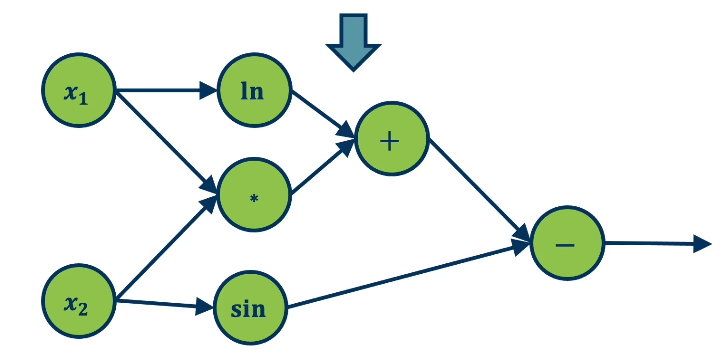

The computation graph can be any directed acyclic graph (DAG), and individual operations within the graph must support differentiation. Mapping operations via a computation graph may seem trivial / excessive in the case of forward propagation, but it is an extremely useful structure for performing gradient descent across all layers within a neural network.

Gradient Descent

Recall that Gradient Descent is an optimization algorithm used to identify the best set of weights with respect to some loss function using derivatives. Computing partial derivatives for each parameter in the context of neural networks seems a bit tricky, though. How can we do this efficiently?

Backpropagation

Backpropagation computes the partial derivative of loss with respect to each parameter in the network by recursively applying the chain rule of calculus to the network’s computation graph. Backpropagation starts at the end of the network (loss function), performing a backwards pass through each layer to update weights.

For any module within the network, we have three terms of interest.

• Partial derivative of loss w.r.t. module output $\frac{\partial{L}}{\partial{h^{\ell}}}$
• Partial derivative of loss w.r.t. weights of layer $\frac{\partial{L}}{\partial{W}}$
• Partial derivative of loss w.r.t. module input $\frac{\partial{L}}{\partial{h^{\ell - 1}}}$

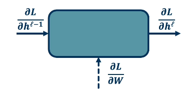
The gradient with respect to module output is given to us by the previous iteration of backpropagation (on the first iteration, we simply compute the gradient of the loss with respect to the preceding layer). For each module, we are tasked with computing…

• $\frac{\partial{L}}{\partial{W}} \rightarrow$ used to update the weights of the layer.

\[\frac{\partial{L}}{\partial{W}} = \frac{\partial{L}}{\partial{h^{\ell}}} \times \frac{\partial{h^{\ell}}}{\partial{W}}\]

• $\frac{\partial{L}}{\partial{h^{\ell - 1}}} \rightarrow$ not directly used to update the weights of the layer, but instead necessary for continuing to propagate the gradient backwards through the network. Becomes $\frac{\partial{L}}{\partial{h^{\ell - 1}}}$ for the next iteration of backpropagation.

\[\frac{\partial{L}}{\partial{h^{\ell - 1}}} = \frac{\partial{L}}{\partial{h^{\ell}}} \times \frac{\partial{h^{\ell}}}{\partial{h^{\ell - 1}}}\]

Therefore, our primary interest is to compute the local gradients $\frac{\partial{h^{\ell}}}{\partial{W}}$ and $\frac{\partial{h^{\ell}}}{\partial{h^{\ell - 1}}}$ and applying them as part of the chain rule. Why is the chain rule relevant here? If our network consists of the following functions…

1. Layer 1: $h_1 = \sigma(XW_1^T + b_1)$
2. Layer 2: $h_2 = \sigma(H_1W_2^T + b_2)$
3. Output Layer: $o = \text{Softmax}(H_2W_3^T + b_3)$
4. Loss Function: $L$

… we really have a composition of functions.

\[L(o(h_2(h_1(X))))\]

Whenever we have a composition of functions, we can compute the derivative of the inner portions of the function w.r.t. the output by multiplying intermediate local derivatives.

\[\frac{\partial{L}}{\partial{W_1}} = \frac{\partial{L}}{\partial{o}} \times \frac{\partial{o}}{\partial{h_2}} \times \frac{\partial{h_2}}{\partial{h_1}} \times \frac{\partial{h_1}}{\partial{W_1}}\]

Note that the computation of the gradient for the weights in the earliest layer $W_1$ is not dependent on the gradient of any other weights in the network, but rather the incoming gradient of the loss with respect to the layer’s output.

Once we have the gradient for each parameter in the network, we can update the parameter value using the gradient descent update rule.

\[w_i^{(t+1)} = w_i^{(t)} + \alpha\frac{\partial L}{\partial w_i}\]

Automatic Differentiation

While backpropagation gives us a method for computing the gradient of the loss w.r.t. each model parameter, it can be applied in many (potentially inefficient) ways. Note that we must store intermediate calculations when performing backpropagation:

• Layer Activations: necessary to compute the local gradient for weights.
• Gradient w.r.t. Input: necessary to continue backpropagating loss to earlier layers.

Reverse-Mode Automatic Differentiation is an efficient implementation of the chain rule on computation graphs. As part of Auto-Diff, we decompose our function composition into a series of primitive operations (ex: multiplication, addition, division, etc.) to form the computation graph. Our Auto-Diff engine should be able to compute derivatives for these simple operations. By breaking down the function into primitives, we avoid the case of pure symbolic differentiation - computing the derivative specific to an individual and perhaps complicated function.

We trace the computation graph starting from the loss, computing and storing the gradient at each node, until reaching our model parameters of interest. During the preceding forward pass, we must store intermediate activations at each node to compute the gradient as necessary.

The flow of gradients backwards through the computation graph is the most important aspect of learning. Different function types (ex: multiplication, addition, max operation, etc.) result in different gradient operations; therefore, choice of function certainly impacts gradient flow.

Forward-Mode Automatic Differentiation takes a similar approach, but starts at the input layer of the computation graph and propagates gradients forward. Forward Auto-Diff tracks the derivative of all intermediate variables with respect to one input parameter at a time. This is extremely inefficient in the case of deep learning, since we require a separate forward pass for each input parameter.

Vectorization

Both forward and backpropagation require a substantial amount of matrix multiplication. By making use of parallelized hardware such as Graphics Processing Units (GPUs) via vectorization, these operations can be made to be extremely efficient.

---

(all images obtained from Georgia Tech DL course materials)