DL M3: Optimization of Deep Neural Networks

Review of Deep Learning

Gradient Descent and Neural Networks

Recall that Backpropagation - otherwise known as reverse-model automatic differentiation (synonymous in the context of machine learning) - is the recursive application of gradient descent to neural network layers via the chain rule of calculus.

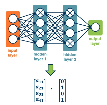
Backpropagation enables us to use any differentiable function as a component of a neural network. For Deep Neural Networks (DNNs) - neural networks with at least two hidden layers - this implies we can select from a wide range of functions for each layer.

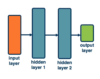
DNN Design Considerations

Since we’ve covered the core components of neural networks, what else is there to consider? Although we have the basic framework in place, there is a huge degree of flexibility to selecting specific implementations of each component.

• Architecture: structure of hidden layers + functions influences the network’s ability to represent a given task.
• Data: preprocessing steps such as normalization / augmentation can improve the quality / quantity of data, and thus improve model performance.
• Training and Optimization: optimization algorithms can be tweaked in many different ways to fit characteristics specific to the task at hand.
• Machine Learning Considerations: networks should be designed to effectively balance model bias vs. variance, and mitigate issues such as overfitting.

In this module, we will explore each of these sub-domains to ensure we make informed decisions when designing our own neural networks.

DNNs: Architectural Considerations

Architecture?

The Architecture of a neural network specifies its composition in terms of 1) module (hidden layer) function types, and 2) connections between different modules. Certain compositions provide architectural bias to better fit the characteristics of a certain problem type. For example, top-performing architectures for natural language processing (NLP) problems tend to differ from those for computer vision (CV) problems.

High-Level Architectures

Example neural architectures include…

• Fully-Connected Neural Networks: use dense connections between layers, where each node in the previous layer is connected to each node in the subsequent layer.
  • this can be computationally excessive for certain problem types.
• Convolutional Neural Networks (CNNs): connections are sparse such that output nodes are influenced by a small window of input nodes.
  • particularly useful for problems involving local structures, such as image tasks.
• Recurrent Neural Networks (RNNs): processes variable-sized inputs in an iterative fashion, using information from previous steps as input to the current step (alongside the actual input).
  • suitable for sequence data such as natural language.

The first step to neural architectural design is always to understand your data - architectural choices should be guided by the type of data used and its characteristics.

Module Types

DNNs consist of a sequence of alternating linear and non-linear layers.

• Linear: $w^Tx$
• Non-linear (example): $\frac{1}{1 + e^{-x}}$

Note that a combination of linear layers alone would have the same representational power as a single linear layer. For this reason, non-linear layers are crucial to increasing representational power.

\[w_1^Tw_2^Tw_3^Tx = w_4^Tx\]

While gradient flow across linear layers is relatively straightforward, flow across non-linear layers is much more variable. Function characteristics such as gradients at extreme points and computational complexity are important considerations for selecting non-linearities.

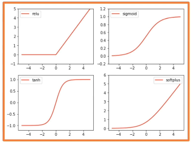
• Sigmoid: $\sigma(x) = \frac{1}{1 + e^{-x}}$
  • becomes saturated at both ends such that gradients become practically zero.
  • therefore, may have issues with vanishing gradients, where learning is hindered by very small gradient flow during backpropagation.
• Hyperbolic Tangent: $\tanh(x) = \frac{1 - e^{-x}}{1 + e^{-x}}$
  • zero-centered, negative values can be learned to flip features.
  • also saturates at both ends, so subject to the same vanishing gradient problem.
• Rectified Linear Unit (ReLU): $\text{ReLU}(x) = \max(0, x)$
  • no saturation on the positive end; no vanishing gradients.
  • ReLU with many negative inputs - “dead ReLU” - may result in poor learning.
  • computationally cheap!

Although no single non-linearity is best for all problem domains, ReLU is the most common starting point due to its low computational complexity and robustness to vanishing gradients.

DNNs: Data Considerations

Relative to other machine learning subfields, deep learning is interesting in that explicit feature engineering is not required. Instead, raw input data drives the learning of both intermediate features and the target function. This makes the characteristics of the input data even more important. We can alter these characteristics to be more appropriate for DNN training.

Normalization

Feature Normalization is the process of transforming numerical features to a common scale to guarantee well-behaved statistics (e.g., range, mean, variance). Normalization can have a tangible impact on gradient-based learning - we can use normalization to ensure activations fall within a desired range, which results in gradients falling within a desirable (i.e., non-saturated) region of non-linear function domains.

Common types of normalization techniques include…

• Standardization: scale feature to standard normal distribution. $s = \frac{x - \mu}{\sigma}$
• Min-Max Scaling: scale feature based on minimum and maximum values. $s = \frac{x - \min}{\max - \min}$

In the context of deep learning, we can implement standardization using layers. This is not problematic so long as the standardization technique is differentiable.

• Batch Normalization: perform standardization for each feature within a mini-batch being passed through the network. For each dimension $d$ of each batch $m \times D$…
  • as part of vanilla standardization, we compute statistics relative to the batch and use them to calculate outputs $s = \frac{x - \mu_{\text{batch}}}{\sigma_{\text{batch}}}$
  • we also introduce learnable parameters into the standardization process to provide the model with more flexibility $y = \gamma s + \beta$
  • during training, we compute batch statistics depending on the training data. during inference, we use stored batch statistics from training and apply them to our data.
• Layer Normalization: repeat same process as for batch normalization, but perform standardization on a per-instance as opposed to per-feature basis. This implies that statistics are computed across all features for each instance.

Once again, normalization is especially important before non-linearities to prevent extremely low and extremely high activation values. This is one method to combat against saturation, which would could result in vanishing / exploding gradients.

Data Augmentation

Augmentation is used as a pre-processing step to transform data in a synthetic fashion. This may benefit model training in terms of 1) training data size, and 2) training data robustness.

In the context of images, here are a few examples of data augmentation:

• Random cropping.
• Flipping the image horizontally / vertically.
• Adding a color jitter - random value added to each color channel.
• Applying geometric transformation - translation, rotation, shear, scale.
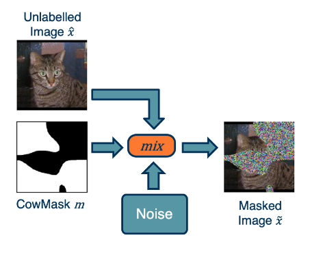
• CowMix: use pixel-wise mask to blend original image with noise or second image.

The more variability provided to the neural network during training, the more generalizable it will be to out-of-sample instances.

DNNs: Optimization Considerations

Weight Initialization

Furthermore, we might be interested in using different weight initialization techniques depending on the problem. Initial parameter values have a massive impact on learning since parameter values directly influence gradients. For example…

• If weights are initialized to large values, activations (intermediate outputs from hidden layers) will also be large.
• If activations are large, the gradients for non-linearities (ex: sigmoid, tanh) may come from saturated regions of the function’s domain. This will limit learning.

Ideally, weights should be initialized such that activations fall within “normal” regions of the non-linearities. A common approach is to initialize weights to small normally distributed random values.

DNNs may still struggle with small initial parameter values - the depth of the network implies many products of activation $\times$ upstream gradient, and small activations will therefore limit gradient-based learning. DNNs must therefore balance the competing issues of saturation and small activations.

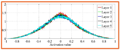
Perhaps the most ideal approach is Xavier Initialization, which samples weight values from a uniform distribution dependent on hidden layer size (number of nodes). This is an ideal approach since it maintains the variance of the output as similar to the variance of the input.

\[\text{Uniform}(-\frac{\sqrt{6}}{\sqrt{n_j + n_{j+1}}}, + \frac{\sqrt{6}}{\sqrt{n_j + n_{j+1}}})\]

• $n_j$ is the fan-in: number of incoming nodes connected to a given node.
• $n_{j+1}$ is the fan-out: number of output nodes connected to a given node.

Choice of Optimizer

Recall that our optimization problem is to identify the set of weights that minimizes our loss function. In the context of deep learning, an Optimizer is a specific optimization algorithm which aims to find our ideal set of weights.

There are many challenges to consider during the optimization process:

• Deep learning involves complex, compositional, non-linear functions, which results in a highly non-convex loss function.
• Saddle Points - locations on the loss surface where the gradient of orthogonal directions is 0 - can cause slow learning or gradients to become “stuck”.
• Gradient estimates are noisy in the case of stochastic gradient descent (SGD).

Different optimizers incorporate different strategies to combat these problems:

• Momentum: rather than updating by the negative gradient, we calculate some velocity term based on the combination of the previous and current gradients. This means the gradient will continue moving in the direction it moved in previously!
  • velocity is an exponential moving average of the gradient
  \[v_i = \beta v_{i-1} + \frac{\partial L}{\partial{w_{i-1}}}\] \[w_i = w_{i-1} - \alpha v_i\]
  • this strategy is particularly useful for 1) faster convergence, and 2) overcoming saddle points.
  • Nesterov Momentum is a variant of momentum which updates weights with the previous velocity term prior to computing the gradient + updating weights again.
  \[\hat{w}_{i-1} = w_{i-1} + \beta v_{i-1}\] \[v_i = \beta v_{i-1} + \frac{\partial L}{\partial{\hat{w}_{i-1}}}\] \[w_i = w_{i-1} - \alpha v_i\]
• Second-Order Methods: gradient descent is a first-order optimization method, meaning we utilize the first derivative of the loss function with respect to each weight (Jacobian). Second-order optimization methods utilize the second-order derivatives of the loss function with respect to each weight (Hessian).
  • this provides us with information about the curvature of the loss function, which can be combined with Taylor Series Expansion to more efficiently jump to the minima of the loss function.
  • the Hessian also indicates how “difficult” the loss function is - the condition number is calculated as the ratio between the smallest and largest eigenvalues, which indicates the difference in curvature along different dimensions. A high condition number corresponds to big steps in some dimensions and small steps in others.
• Per-Parameter Learning Rates: assign a dynamic learning rate to each weight. Examples include…
  • Adagrad: gradient statistics inform learning rate reduction across iterations. As gradients accumulate (represented by $G_i$), learning rate goes to zero. This means weights with larger gradient values will have a learning rate proceed to zero faster than weights with smaller gradient values.
  \[G_i = G_{i-1} + (\frac{\partial{L}}{\partial{w_{i-1}}})^2\] \[w_i = w_{i-1} - \frac{\alpha}{\sqrt{G_i + \epsilon}} \cdot \frac{\partial{L}}{\partial{w_{i-1}}}\]
  • RMSProp: instead of using the sum of gradients across iterations, keep a moving average of squared gradients. This avoids premature saturation of learning rate to zero. \(G_i = \beta G_{i-1} + (1 - \beta)(\frac{\partial{L}}{\partial{w_{i-1}}})^2\)
  • Adam: combines the ideas of momentum and RMSProp to yield a composite algorithm. Since initial values for $v_i$ and $G_i$ might be unstable (e.g., close to zero), we can use a time-varying correction to ensure we don’t have issues at the start of learning.
  \[v_i = \beta_1 v_{i-1} + (1 - \beta_1)(\frac{\partial{L}}{\partial{w_{i-1}}})\] \[G_i = \beta_2 G_{i-1} + (1 - \beta_2)(\frac{\partial{L}}{\partial{w_{i-1}}})^2\] \[\hat{v}_i = \frac{v_i}{1 - \beta_1^t} ~~~~~ \hat{G}_i = \frac{G_i}{1 - \beta_2^t}\] \[w_i = w_{i-1} - \frac{\alpha v_i}{\sqrt{G_i + \epsilon}}\]

Each of these optimizers behave differently depending on the surface of the loss function. Undesirable behaviors such as overshooting or stagnating may still occur. Vanilla SGD with Momentum can generalize better than adaptive methods, but may require a higher degree of tuning.

Regularization

In the context of machine learning, Regularization refers to a broad class of methods for reducing overfitting during model training. Recall that overfitting refers to the situation where a model fits noise in the training data as opposed to the underlying trend we wish to represent. Overfitting is typically signaled by a significant gap in performance between training and validation data, where generalization error is much higher than training error.

Many regularization methods apply some additional penalty to the loss function based on the magnitude of the current weights:

• L1 Penalty: sum of the absolute values of the weights.
  • encourages sparsity = few non-zero values.

\[L = |y - Wx_i|^2 + \lambda|W|\]

• L2 Penalty: sum of the squared values of the weights.

\[L = |y - Wx_i|^2 + \lambda |W|^2\]

• Elastic Penalty: linear combination of L1 and L2 penalties.

\[L = |y - Wx_i|^2 + \alpha|W|^2 + \beta |W|\]

Penalty-based regularization tends to produce smaller weight values. Since smaller weights result in smaller model variance, this is one technique for mitigating overfitting.

Other regularization methods apply to neural networks specifically. Dropout is a technique which probabilistically removes (“drops”) a certain percentage of nodes in a neural network layer during each iteration of training. This process forces the network to learn more robust features and representations that do not rely on any particular subset of nodes. Dropout is practically implemented by masking activations of deactivated nodes to zero.

At inference time, we do not perform any dropout. Instead, we may scale the weights at train or inference time by some term involving dropout probability. This helps to ensure activation distributions are similar at train versus inference time.

DNNs: Training Considerations

Training deep neural networks is more of an art than a science. Many different factors contribute to the final outcome - the goal is to find a combination of components that works particularly well, where there exists a reasonable number of reasonable combinations.

General Methodology

Properly executed DNN Training should split input data into the following partitions:

• Training Set: used to directly optimize model weights.
• Validation Set: used to select hyperparameters / architectures / optimizers.
• Test Set: used to estimate generalization (out-of-sample) performance.

Cross-Validation is an alternative procedure which may be used in place of a validation set. Instead of holding out a dedicated validation set, the training set is divided into $k$ folds, where $k-1$ folds are used for training and the $k$-th fold is used to estimate validation performance. Each possible combination of training : validation folds is used to train : evaluate the model, then evaluation metrics are summarized across iterations. This method is computationally expensive, and should only be used in the case of relatively small data.

Metrics + Monitoring

The key to DNN Training is to monitor many different metrics to understand what is happening during training. So what metrics should we be looking at?

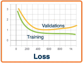
• Loss / Accuracy Curves: plot loss or accuracy as a function of training iteration (iteration may be per-batch or per-epoch). Should be plotted for both training and validation data splits.
  • Training + validation loss constant across iteration $\rightarrow$ major problem with learning.
  • Training loss decreases, but validation loss is constant $\rightarrow$ model is overfitting.
  • Training + validation loss decreases slowly $\rightarrow$ learning rate is too small.
  • Training + validation loss increases $\rightarrow$ learning rate is too large.
• Learning Curve: somewhat vague, but tends to describe a curve of training + validation performance as a function of training data size. Typically used to evaluate the impact of increasing / decreasing training data size on model performance.
  • Validation loss shows decreasing trend through end of plot $\rightarrow$ more training data would be useful in further improving model generalization.

Recall the difference between overfitting and underfitting in machine learning. Overfitting is the case where validation loss diverges from training loss, where training loss continues to improve while validation loss remains constant or increases. Our model may have too much variance as compared to bias.

Conversely, Underfitting is the case where training and validation loss are both very close, and perhaps relatively poor. Our model may benefit from additional variance.

Hyperparameter Search

A Hyperparameter is any value which influences a model’s representation, but is not directly learned from the data. Hyperparameters should be tuned to the specific dataset in order to match the model’s configuration to characteristics of the problem at hand. Deep learning involves a large number of hyperparameters. These include variables such as hidden layer size, number of hidden layers, learning rate, momentum, and regularization coefficient.

Hyperparameter Tuning is the process of selecting an optimal set of hyperparameters to minimize validation loss. We can perform hyperparameter tuning in a number of different ways:

• Grid Search: iterate over each possible configuration in the hyperparameter search space.
• Random Search: randomly sample from the hyperparameter search space.
• Bayesian Search: use previous iterations of hyperparameter search to probabilistically inform subsequent iterations.

Note that many hyperparameters are inter-dependent, so they cannot be reliably tuned individually.

---

(all images obtained from Georgia Tech DL course materials)