DL M5: Convolutional and Pooling Layers

Introduction

To recap previous lessons, a Deep Neural Network is a machine learning model characterized by two or more hidden layers, where each layer must be some differentiable function. The structure of a neural network can be broken down into two main considerations:

• Architecture: arrangement of layers and connections between layers.
• Layer Type: specific function used to map inputs to outputs for a given layer.

So far, we’ve only covered one neural architecture: the fully-connected neural network (also known as a multi-layer perceptron). This is a network in which 1) all information flows forward to generate the final prediction, and 2) each input node is connected to each output node within each layer.

Other Architectures

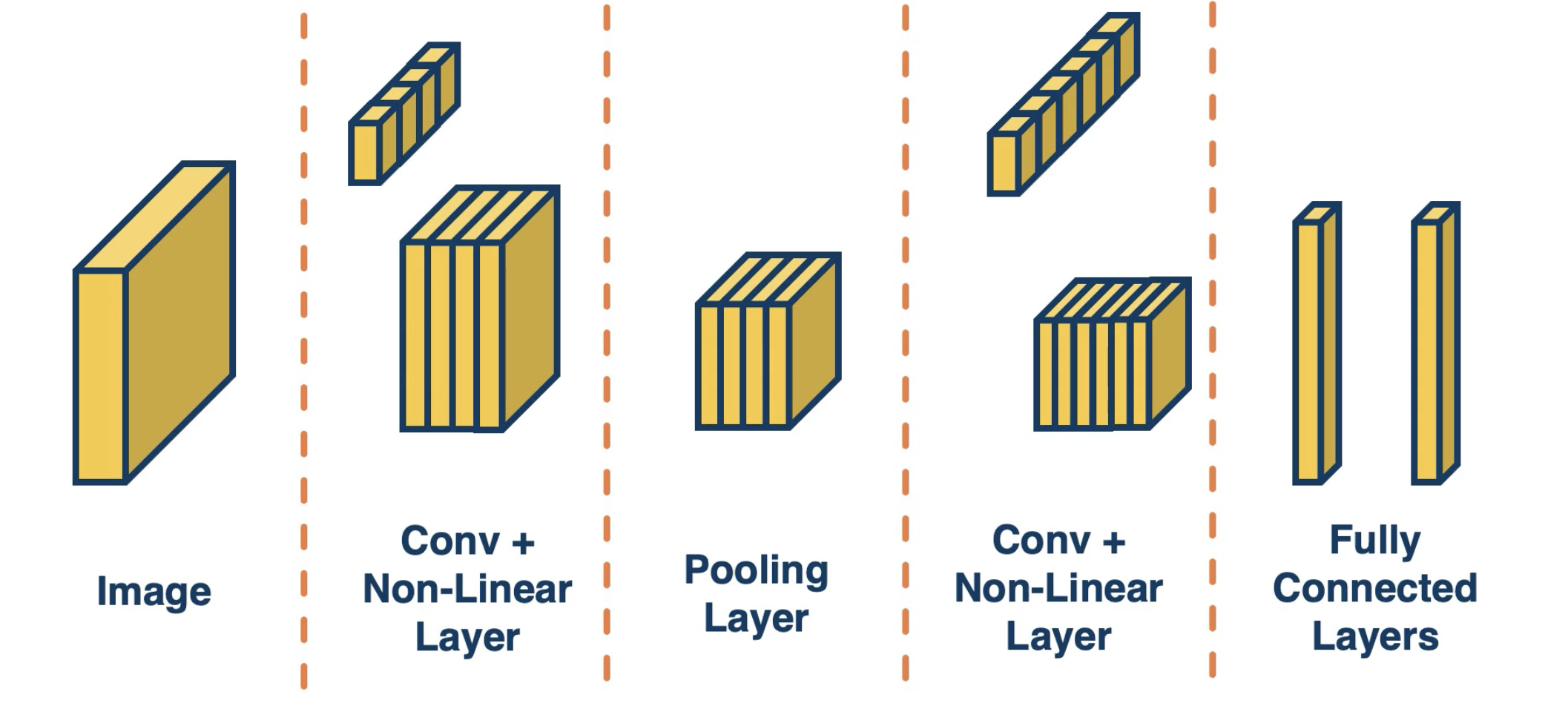
In addition to the fully-connected architecture, there are many alternative approaches for constructing a neural network. For example, Convolutional Neural Networks (CNNs) contain layer types other than the fully-connected layer, including convolutional and pooling layers. CNN architectures are most applicable to data with local structures; this is particularly prevalent when considering image data.

See below for an example of a typical CNN layer arrangement.

Convolutional Layers

Convolutional Layers apply the convolution operation (discussed later) to their input. Unlike fully-connected layers, convolutional layers do not require all possible connections between input and output nodes.

Why not Fully-Connected?

Recall that each fully-connected layer requires a total of $M*N + N$ parameters, where $M$ is the number of input nodes and $N$ the number of output nodes. Given a $1024 \times 1024$ image, we would need over one million parameters for a fully-connected layer with one output node!

Certain task domains (such as image processing) involve spatially-localized features. For example, edges and corners can be detected within smaller patches of an overall image. Furthermore, these features are not specific to any specific region of the input. Convolutional layers introduce an architectural bias into the modeling approach to reflect these characteristics, resulting in a more efficient + effective representation of the task at hand.

What is a Convolutional Layer?

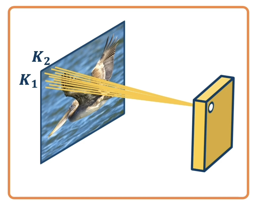
As part of a convolutional layer, each output node is connected to a small portion of the original input called the receptive field. More specifically, we iteratively pass a kernel - a tensor of parameters - over all possible receptive fields in the input. At each iteration, we take the dot product between weights in the kernel and input values in the receptive field, then add some bias term. This produces the corresponding output node in the feature map associated with the kernel.

Consider the below example - our image on the left is the input, our 2D kernel is represented by the $K_1 \times K_2$ window on the image, and the feature map associated with this kernel is on the right. The specific iteration shown maps the top-left receptive field to the top-left region of the feature map.

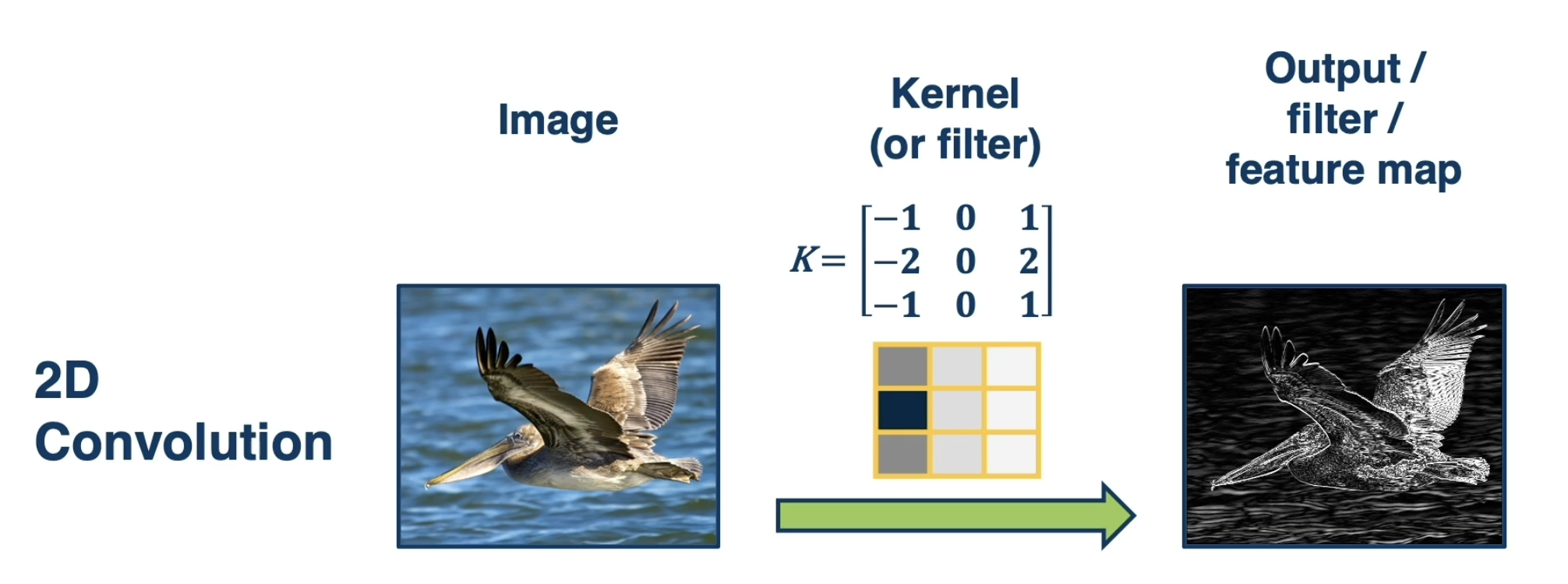
A convolutional layer can have multiple kernels, thus producing multiple feature maps in the output layer. Kernels are typically used as feature extractors in that each kernel is responsible for learning a different aspect of the input image (ex: Kernel 1 $\rightarrow$ edges, Kernel 2 $\rightarrow$ shadows, etc.).

One primary benefit of this approach is parameter sharing. Instead of having a dedicated parameter for each pixel in the input, we have $(K_1 \times K_2 + 1)$ parameters for each kernel used in the convolutional layer. Parameter sharing is not only beneficial for reducing computational overhead, but also for task representation - applying the same set of parameters over all possible regions of the input implies that the location of a particular feature within the input does not matter. In addition to parameter sharing, this representation is useful because it preserves spatial orientation when mapping from input to output.

Ultimately, our goal in using a convolutional layer is the same as a fully-connected layer. We are interested in learning the best set of parameters (now within our kernel) to produce the best predictions for our task.

Convolution vs. Cross-Correlation

The process of striding a kernel along an input is actually a specific implementation of a more general mathematical concept. The convolution operation measures the area of overlap between two functions $f$ and $g$ over their shared domain (set of possible input values), where the second function is reflected before computing overlap. Similarly, cross-correlation involves the same process, but does not flip the second function.

Note that the “convolution” in CNNs is actually cross-correlation, but this distinction is not very important since the kernel involves learned parameters (and thus reflecting the kernel prior to learning does not impact final learned values).

For more on the convolution operation, check out 3Blue1Brown’s Video on the topic.

Hyperparameters

Any convolutional layer has certain hyperparameters defining its configuration:

• in_channels: number of channels (ex: color) in the input.
• out_channels: number of kernels / output feature maps.
• kernel_size: shape of the kernel, specified as a tuple.
• stride: number of pixels to move at each iteration of the convolution.
• padding: zero padding added to both sides of the input.

Input and Output Sizes

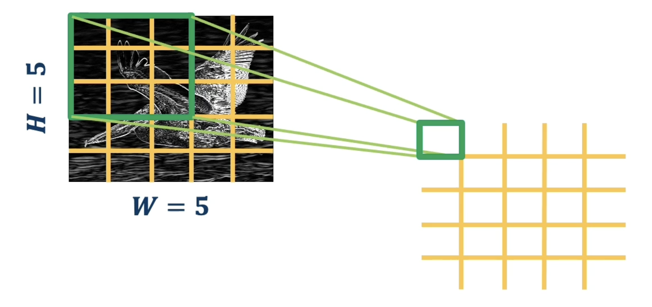
The output size of a vanilla 2D convolution is simply $(H - k_1 + 1) \times (W - k_2 + 1)$. Given a specified stride and zero-padding, this formula changes to: \(H_{\text{out}} = \frac{H_{\text{in}} - k_1 + 2n_{\text{pad}}}{stride} + 1, ~~~ W_{\text{out}} = \frac{W_{\text{in}} - k_1 + 2n_{\text{pad}}}{stride} + 1\) In the case of multi-channel input (ex: 2D images with three color channels $\rightarrow$ $H \times W \times C$), we simply extend our kernel from 2D to 3D. This implies the output size is no different than the single-channel case with a 2D kernel.

Recall that the number of output feature maps is dependent on the number of kernels. With this in mind, our final output size will be $(H_{\text{out}} \times W_{\text{out}} \times O)$, where $O$ is the number of kernels and each $(H_{\text{out}} \times W_{\text{out}}$) slice is a distinct feature map.

Pooling Layers

Pooling Layers are also commonly found in CNNs. The primary purpose of a pooling layer is to perform dimensionality reduction, reducing the size of the input via some specified method. Similar to convolutional layers, pooling layers iterate over all possible receptive fields in the input, but perform some summary operation within each receptive field. This implies that pooling layers do not have learnable parameters.

For example, consider a Max Pooling Layer. At each iteration, max pooling takes the maximum of the receptive field to yield a single output value. In addition to the maximum operation, we can use any differentiable function as part of a pooling layer as to stay compatible with backpropagation.

Hyperparameters

Any pooling layer has the following hyperparameters:

• kernel_size: the size of the window to perform the operation over (ex: max).
• stride: the stride of the window, with a default of kernel_size.
• padding: zero padding added to both sides of the input.

Role within CNNs

The combination of sequential convolutional and pooling layers results in translational invariance - a property in which slight translations (movement) of input features result in the same output value. Convolutional layers also have translational equivariance, which states that movements in the input will be reflected as corresponding movements in the output. This property is not associated with the pooling operation.

---

(all images obtained from Georgia Tech DL course materials)