DL M7: CNN Visualization

Introduction

Given a trained convolutional neural network (CNN), how can we understand what it has learned? The key idea of this lesson is that we can visualize different aspects of a CNN (intermediate outputs, kernel, gradients, etc.) to gain insight into what’s going on under the hood.

CNN Visualization Strategies

Kernel Weights

For any Convolutional Layer, we can visualize the kernel weights by scaling the weights to values from $[0, 255]$. Recall that weights are initialized to random values; the final learned weights might reveal insight into the structure of a particular learned feature extractor.

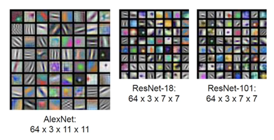
This process isn’t always ideal, considering kernels tend to be small (ex: $3 \times 3$).

Intermediate Outputs

Recall that a convolutional layer produces Feature Maps as output; given an input and kernel (feature extractor), the output represents the final extracted features. We can visualize convolutional activations to understand what aspects of the input are preserved / highlighted as a result of the convolution operation. Consider the following example, which seems to indicate that the given CNN kernel has learned to extract information on faces.

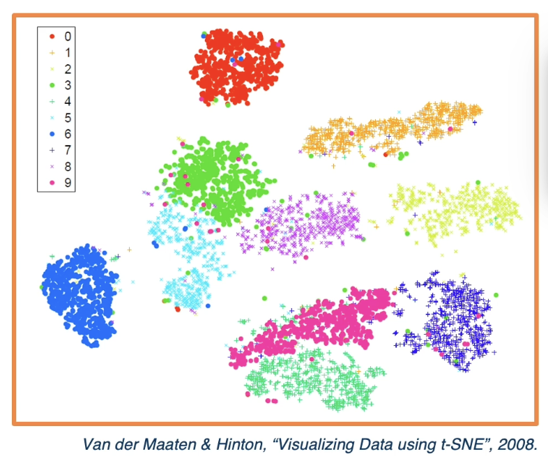
Other approaches for visualizing activations include performing dimensionality reduction into a smaller dimensionality for plotting. For example, we may use approaches like Principle Component Analysis (PCA) or t-SNE to prepare high-dimensional activations for 2D plotting.

Gradient-Based Visualizations

In previous lessons, we saw how to calculate the gradient of the loss w.r.t. the weights of each layer in order to perform gradient descent. We can also calculate the gradient of the loss w.r.t. our original inputs $\frac{\partial{L}}{\partial{X}}$via a similar process. Okay, but why would we even want to do this?

$\frac{\partial{L}}{\partial{X}}$ indicates the sensitivity of loss w.r.t. individual pixels, where a larger sensitivity implies more important pixels. Visualizations based on $\frac{\partial{L}}{\partial{X}}$ are called Saliency Maps.

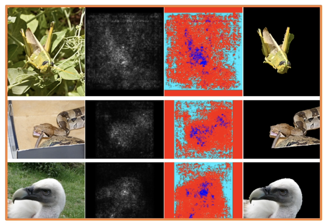
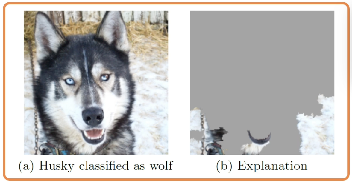
Saliency maps are a useful tool for determining which regions of an input image are used during model inference. Additionally, they can be used to detect dataset bias - if our result highlights pixels that SHOULD NOT be important for the final prediction, we know our model has learned a problematic representation.

The gradient w.r.t. an input image can also be used to generate new images via gradient ascent. More specifically, we can update the pixels of the original image by using the gradient for a specific class, thereby increasing the network’s likelihood of classifying the image as that class.

Other Considerations

Robustness

The Robustness of a CNN refers to its ability to confidently predict the correct class despite slight perturbations to the input image. Research has shown that adversarial attacks such as single-pixel changes or random noise perturbation can greatly change the output confidence of a CNN; even if the altered image looks similar from the perspective of human eyes!

Similar to other security-related areas of computer science, this is a cat-and-mouse game. Neural networks cannot be fully robust to every single attack type; as new attacks are launched, new defense mechanisms are developed.

We can also try to understand the biases of CNNs and compare them to human intuition. One common example of this is a shape vs. texture bias analysis - given an image of one class retextured to represent another class, which class does the network predict?

Style Transfer

Style Transfer is an image generation process which preserves the content of a given image, but alters style to match another image.

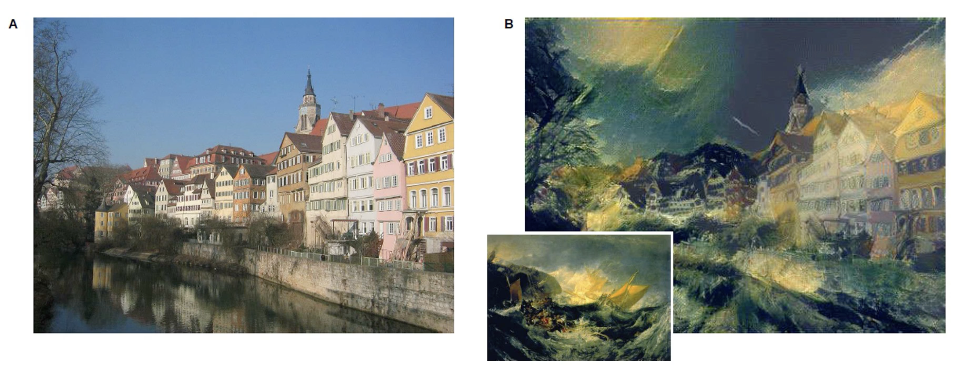
Style transfer is accomplished by altering the loss function to match our goals. Researches have found we can represent texture similarities via feature correlations. The Gram Matrix computes correlations between all pairs of feature maps in a convolutional output. We denote the Gram Matrix for a particular convolutional layer $\ell$ as $G^{\ell}$.

\[G^{\ell}_{(i,j)} = \sum_k F^{\ell}_{(i,k)}F^{\ell}_{(j,k)}\]

Given the Gram Matrices for each convolutional layer of a style network, we can calculate loss as the difference relative to every corresponding Gram Matrix in our target network. Total loss for a target network is therefore a combination of content-based loss and style-based loss.

\[L_{\text{style}} = \sum_{\ell}(G^{\ell}_{\text{final}} - G^{\ell}_{\text{style}})^2\] \[L_{\text{total}} = \alpha L_{\text{content}} + \beta L_{\text{style}}\]

---

(all images obtained from Georgia Tech DL course materials)