DL M9: Introduction to Structured Representations

Introduction

So far, we’ve talked about two neural Architectures, where architecture refers to the composition of modules within a neural network.

• Fully Connected Neural Networks: alternation of dense linear layers and element-wise non-linear transformations.
• Convolutional Neural Networks (CNNs): utilize convolutional and pooling layers, which do not involve dense mappings between every pairing of input and output nodes.

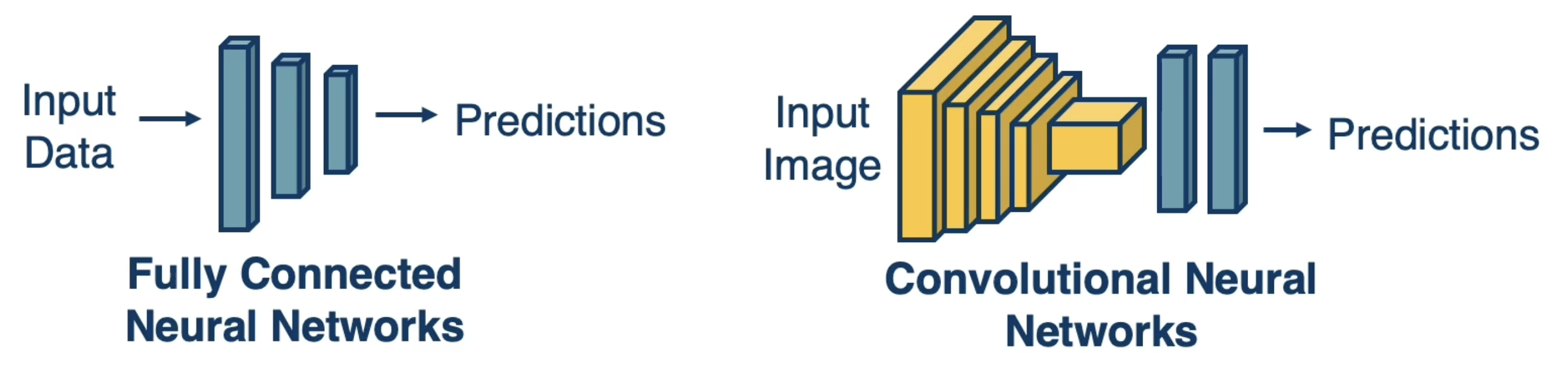
Note that CNNs make use of architectural bias - a design component of the neural network that influences representational learning - to take advantage of characteristics specific to the target problem (e.g., computer vision). Image-based tasks are highly dependent on local structure, and convolutional layers are efficient + effective at learning features for local structure.

The notion of architectural bias is not specific to CNNs / computer vision. In fact, there are many other neural architectures which utilize architectural bias to match the respective data structures corresponding to their problem types.

Architecture Types

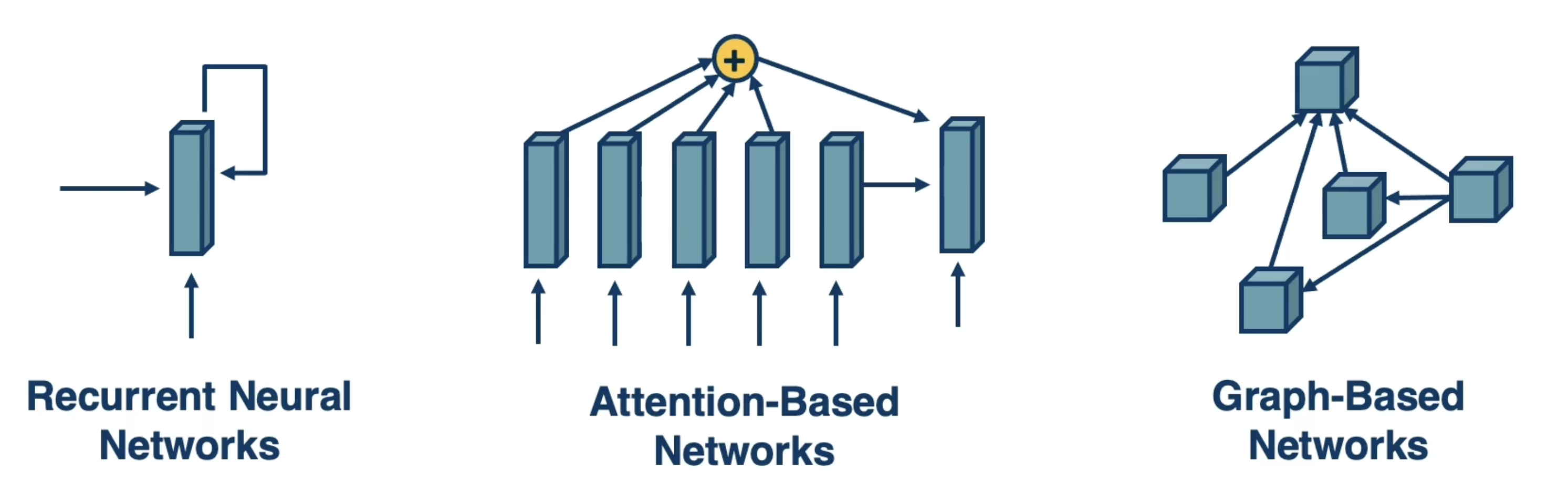
Recurrent Neural Networks

Recurrent Neural Networks (RNNs) make use of recurrent structure to fit sequential data, which is especially prevalent in the field of natural language processing (NLP). For a given input sequence, the recurrent unit processes each time step sequentially, and maintains some hidden state vector to utilize information from previous time steps in the prediction for a current time step. Similar to CNNs, RNNs take advantage of parameter sharing since the same weights in the recurrent unit are applied for each time step.

Fully connected neural networks struggle when applied to sequence data since they require fixed-size inputs; the number of input features should match the number of terms in the sequence. RNNs offer a more flexible and efficient means to processes sequence data, enabling variable-length sequences to be valid input for the the same network.

RNNs do come with certain limitations. They are particularly prone to optimization issues such as the vanishing / exploding gradient problem, which tends to happen for long sequences of data. Furthermore, a single hidden state vector may not be able to accurately represent all relevant information from previous time steps.

Attention-Based Networks

Attention (Attention Is All You Need, 2017) addresses many limitations of RNNs. Attention is a neural mechanism which weights other terms of an input sequence for use in the current prediction. In contrast to a single hidden state vector, this enables dynamic “attention” to different portions of the input as considered relevant by the network.

Transformer architectures use attention-based modules as building blocks (more specifically, multi-headed attention) to achieve state-of-the-art performance on many language problems.

Language Modeling

One key application of sequential modeling is Language Modeling - what is the probability of observing a particular sequence of words in natural language?

Representing Language as an ML Problem

We can model any word in a sequence as a factorized probability distribution via the product rule of probability:

\[\Pr(w_1, \ldots, w_n) = \prod_i \Pr(w_i | w_{i-1}, \ldots, w_1)\]

Text generation iteratively models the probability of observing each possible next word $w_i$ given a historical sequence $w_{i-1}, \ldots, w_1$.

Instead of predicting words, we may also be interest in generating a meaningful semantic representation of text. Word Embeddings are vectorized representations of words created by neural networks which learn patterns based on word context, usually by training on distributional semantics via skip-gram models. Word2vec and BERT are examples of popular word embedding networks.

Structures and Structured Representations

Neural Networks and Architectural Bias

We have seen how to build and optimize deep feedforward architectures consisting of linear and non-linear (e.g. ReLU) layers. Optimization procedures such as Backpropagation and automatic differentiation can be applied to arbitrary computation graphs, regardless of architecture. This is apparent in the case of CNNs.

Most problems in deep learning have hierarchical composition. Depending on the problem type, hierarchies may look slightly different:

• Computer Vision: pixels $\rightarrow$ edge $\rightarrow$ texton $\rightarrow$ motif $\rightarrow$ part $\rightarrow$ object.
• Speech: sample $\rightarrow$ spectral band $\rightarrow$ formant $\rightarrow$ motif $\rightarrow$ phone $\rightarrow$ word.
• Language: character $\rightarrow$ word $\rightarrow$ NP/VP/PP $\rightarrow$ clause $\rightarrow$ sentence $\rightarrow$ story.

It turns out we can introduce certain architectural biases into neural network structure to fit the characteristics of a given problem type. This facilitates more effective representation / modeling of the true relationships in our data.

Structured Representation

The term Structured Representation refers to the neural architectural design choices of a particular structure intend to represent characteristics of a problem type. Structured representations may be specific (ex: RNNs to sequence data), or general (ex: graph networks in which structure is learned).

When representing structured information, several components are important:

• State: compactly represents all data we have processed thus far.
• Neighborhoods: what other elements should be considered for a given instance?
• Propagation of Information: how can we update our collective “information” (hidden state) given important elements?

Attention

Attention is one of the most important neural mechanisms for propagating information based on neighborhoods of elements. The attention mechanism performs a weighted sum over candidate elements in a set, where weights are calculated via some relevance metric such as embedding similarity.

Given a set of key vectors $\begin{Bmatrix} k_1, \ldots, k_n \end{Bmatrix}$ and a query vector $q$ …

1. Calculate attention weights as softmax-ed cosine similarity between query vector and keys.

   \[a_j = \frac{e^{k_j \cdot q}}{\Sigma_i e^{k_i \cdot q}}\]

2. Define final state vector as weighted sum of attention weights and values corresponding to each key $\begin{Bmatrix} v_1, \ldots, v_n \end{Bmatrix}$

\[\text{output} = \Sigma_i a_i v_i\]

This mechanism is very powerful because it enables representation of arbitrary sets of information in a dynamic fashion. Attention can be applied within many different neural architectures such as RNNs or graph networks.

---

(all images obtained from Georgia Tech DL course materials)