HPC M1: Locality

What’s the Problem?

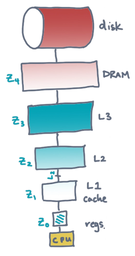
Machines have memory hierarchies, meaning there are structured levels of memory between a processor (e.g., CPU) and primary storage device (e.g., disk). As we approach the processor, the size of memory decreases while the speed of access increases.

The operating system (OS) may automatically manage memory resources effectively for your program. However, optimal resource usage is difficult. The purpose of this lesson is to review methods and algorithms that a programmer may implement to manually take advantage of memory resources.

Basic Locality Models

Two-Level Memory

In order to design a locality-aware algorithm, we must first specify our machine model. We will cover a basic model with inspiration from the Von Neumann architecture.

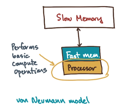
• Processor performs basic compute operations in sequential fashion. Operations might include addition, subtraction, branches, etc.
• Processor is connected to a primary source of memory $\rightarrow$ Slow Memory. This memory is massive, but comes with the cost of high access latency.
• In between the processor and primary memory source is a faster memory cache $\rightarrow$ Fast Memory. This memory has much smaller size and much lower latency.

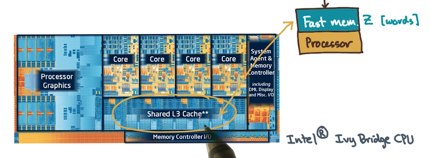
On a real-world processor, the fast memory might be a last-level cache sitting between slower main memory (RAM) and the processor.

There are two rules for computation as part of this model:

1. Local Data Rule $\rightarrow$ Processor may only compute with operands present in fast memory.
2. Block Transfer Rule $\rightarrow$ Transfers from slow to fast memory occur in blocks of size $L$. This implies we cannot perform transfers at the level of a single memory address.

We therefore define Computational Cost in terms of two key components:

• Work $W(n)$ $\rightarrow$ number of computation operations, as a function of input data size.
• Transfers $Q(n; Z, L)$ $\rightarrow$ number of $L$-sized transfers from slow to fast memory.
  • $Z$ is the size of the fast memory.

Practically, we have many possible pairings of slow-fast memory which are therefore considered two-level systems.

• Hard Disk : Main Memory (RAM)
• L1 Cache : CPU Registers
• Remote Server RAM : Local Server RAM
• Internet : Your Brain :)

Example 1: Reduction

We define reduction as any higher-level operation collapsing an array into a scalar value. One example of reduction is summing elements of an array.

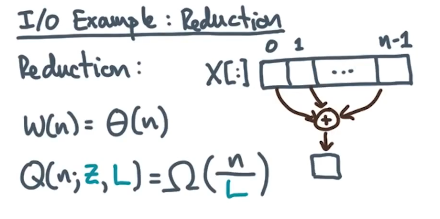
Can we design a reduction algorithm to achieve our lower bound on transfer cost?

for $i \leftarrow$ 0 to $n-1$ by $L$ do:
  local $L \leftarrow \min(n, i + L - 1)$
  local $y[0:L-1] \leftarrow X[i:(i + L - 1)]$
  for $j \leftarrow 0$ to $L - 1$ do $s \leftarrow s + y[j]$

Example 2: Matrix-Vector Multiplication

Given we are interested in optimizing matrix-vector multiplication, how should we define a transfer-efficient algorithm? Assume data is aligned in column-major ordering such that $a_{i,j} = A[i + j \times n]$.

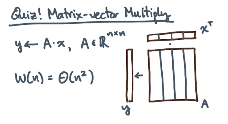
The most memory-efficient way to implement matrix multiplication is to iterate over columns $j$ then rows $i$. This is because the data within columns is proximal (via column-major alignment), and we therefore take advantage of larger transfer hits!

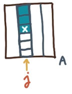
for $j = 0$ to $n-1$ do
  for $i = 0$ to $n-1$ do
    $y[i] += A[i, j] \times x[j]$

Algorithmic Design Goals

What makes an algorithm “good”? First, the algorithm should work optimally. This implies any implementation of the algorithm should do the same asymptotic work as the best local (non-hierarchical memory) case.

\[W(n) = \Theta(W_{*}(n))\]

The algorithm should also achieve high computational intensity, meaning the number of operations per transfer is maximized. Put another way, computational intensity measures the amount of memory re-use as part of your algorithm!

\[\text{Maximize}: ~~ I(n; Z, L) = \frac{W(n)}{L \times Q(n; Z, L)}\]

Consider the relationship between work, transfers, and execution time.

• Suppose the processor takes $\tau$ time units to complete an operation, where $\tau = \frac{\text{time}}{\text{op}}$. We therefore denote total computation time as $T_{\text{comp}} = \tau W$.
• We also define $\alpha$ as the total time required to complete one memory transfer, where $\alpha = \frac{\text{time}}{\text{transfer}}$. This means the total memory transfer time is $T_{\text{mem}} = \alpha L Q$.

We define the total runtime for a program relative to its ideal computation time and penalty associated with memory transfer.

\[T = \tau W \times \max(1, \frac{\alpha / \tau}{W/(LQ)})\]

• The numerator is machine balance $B$ - it indicates how many operations can execute in time it takes to perform a transfer.
• The denominator represents computational intensity $I$.

We can estimate maximum normalized performance via a combination of these terms.

\[R_{\text{max}} = \frac{W_*}{W} \times \min(1, \frac{I}{B})\]

What’s the Point?

Computational analysis in terms of the aforementioned components can help inform architecture when building a new machine. For example, processors may be specialized in terms of machine balance to better facilitate matrix multiplication operations. This is especially helpful for machines performing tasks related to deep learning!

---

(all images obtained from Georgia Tech HPC course materials)