ML M14: Feature Extraction

What is Feature Extraction?

Definition

Feature Extraction refers to the problem of pre-processing a set of features to create a new (perhaps smaller, more compact) feature set, while retaining as much (relevant, useful) information as possible. In this context, we are specifically referring to unsupervised learning techniques such as dimensionality reduction.

\[\mathbf{X} \sim \mathbb{F}^{n} \rightarrow \mathbb{F}^{m} ~~~~ m < n\]

The goal is typically to define some matrix $\mathbf{P}$ to apply a linear transformation to the original feature set, projecting it into a lower-dimensional subspace. The resulting features are therefore linear combinations of the original features!

\[\mathbf{X}_{\text{new}} = \mathbf{X}_{\text{old}}\mathbf{P} ~~~~~ \mathbf{X}_{\text{old}} \in \mathbb{R}^{i \times n}, \mathbf{P} \in \mathbb{R}^{n \times m}, \mathbf{X}_{\text{new}} \in \mathbb{R}^{i \times m}\]

We therefore distinguish feature transformation from feature selection as follows:

• Feature Selection: produce the most informative subset of a feature set without modifying any existing features or creating any new features.
• Feature Extraction: produce the most informative subset of the original features by deriving new features as linear combinations of the original features.

(note that in this lesson, we only consider the subset of feature extraction methods which are considered unsupervised learning and rely on linear transformation. other classes of feature extraction methods may be supervised and/or take a non-linear approach).

What’s the Point?

As consistent with the above definition, we might perform feature extraction as pre-processing for a subsequent end-goal machine learning task. But don’t some of our learning algorithms already perform feature transformation? For example, consider a neural network - we commonly refer to neural nets as feature extractors due to their great ability to learn alternative + informative representations of the original feature set!

Using dedicated feature extraction in conjunction with a learning algorithm (as opposed to bundled into the learning algorithm) may be useful for a number of reasons:

• Feature extraction is performed with an explicit goal in mind (e.g., removing dependent variables), as opposed to being a product of the learning algorithm’s inductive biases.
• Producing a smaller subset of features with similar information may help ease the curse of dimensionality, and increase computational efficiency of the learning algorithm.
• Data can be difficult to visualize in more than a few dimensions; feature extraction is an effective method for preprocessing prior to plotting.

Feature Transformation Methods

PCA

Principal Components Analysis (PCA) reduces a set of features by identifying new features with maximal variance. PCA starts by producing the primary axis - or first principal component - to maximize variance. Projecting the original data points onto this axis produces the highest possible variance. All subsequent axes are selected as mutually orthogonal to the current set. This implies the final set of features is chosen as the top $m$ principal components .

Consider the example below, where our original dataset consists of two features $\mathbf{x}$ and $\mathbf{y}$. The red line represents the first principal component, and maximizes the variance of the projected points.

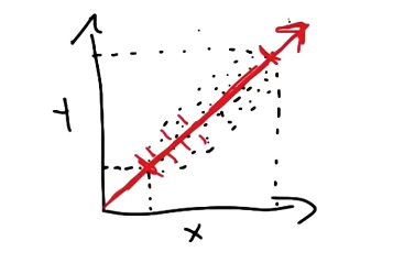
The second component must be orthogonal (perpendicular) to the existing set of components. This means we are very limited in the case of our 2D example!

PCA is guaranteed to yield the best set of features to minimize reconstruction error, which is calculated as the mean squared error between points in the original $\mathbf{X}$ and reconstructed $\mathbf{\hat{X}}$ feature sets.

\[\text{Reconstructed Features}: ~~~\mathbf{\hat{X}} = (\mathbf{XP}_m)\mathbf{P}^T_m\] \[\text{Reconstruction Error}: ~~~ ||\mathbf{X} - \mathbf{\hat{X}}||_F^{2}\]

If we reconstruct using $m = n$ principal components (as in the above image), there will be no reconstruction error; this is because we are simply performing a linear rotation. If we reconstruct using $m < n$ principal components, each subsequent component will be the best possible option to retain information (variance) from the original feature space.

Note that PCA is highly sensitive to feature scale, since features with larger numeric scale may have higher variance as a result. Therefore, it is crucial to apply feature scaling methods prior to PCA.

ICA

Independent Components Analysis (ICA) is similar to PCA, but differs in terms of component selection. PCA functions by selecting new features to maximize variance. Conversely, ICA selects new features to maximize statistical independence. ICA attempts to find a linear transformation of the original feature space such that each of the features in the transformed set are mutually independent.

\[\mathbf{X}_\text{new} \rightarrow \mathbf{x}_i \perp \mathbf{x}_j ~~~\forall i, j\]

Consider the following conceptual representation of ICA. We are given a set of observed variables (current feature set), and tasked with identifying a set of latent (hidden / unobserved) variables which are mutually independent. ICA assumes 1) this set of latent variables exists, and 2) we can generate the target set of latent variables by taking a linear combination of the original feature set.

A real-world example of this scenario is the cocktail party problem, which is a form of blind source separation. Given multiple mixed audio signals from a cocktail party, we are interested in separating the source signal into distinct signals for each of the individual speakers.

As part of the cocktail party problem, the original data-generating sources are independent! Therefore, ICA works great for separating individual audio sources in a mixed recording.

Other Methods

Random Components Analysis (RCA) is similar to PCA and ICA, but selects components (features) in a completely random fashion! Instead of maximizing variance (PCA) or statistical independence (ICA), RCA works by defining new features as random linear combinations of the original feature set. Perhaps surprisingly, this technique is very effective at dimensionality reduction as preprocessing for supervised learning! This is because random projections still maintain some of the original information while helping to reduce the curse of dimensionality. Additionally, RCA is very fast and cheap compared to PCA / ICA due to its simple approach.

Linear Discriminant Analysis (LDA) is a supervised learning approach which finds a projection that discriminates based on a label. Therefore, LDA applies dimensionality reduction as a function of the outcome variable $\mathbf{y}$.

---

(all images obtained from Georgia Tech ML course materials)