ML M17: Reinforcement Learning

What Else?

Reinforcement Learning (RL) implies reward maximization in the context of an agent-environment dynamic. In the previous module, we set the foundation for discussing RL algorithms by defining the following concepts:

• Markov Decision Process (MDP): mathematical representation of a reinforcement learning problem. Core components include environmental state space $S$, action space $A(s)$, state transition matrix $T(s, a, s’) \sim \Pr(s’ | s, a)$, and reward function $R(s)$.
• Bellman Equation: formal definition of state utility given MDP problem components. \(V(s) = R(s) + \gamma \max_a \sum_{s'}T(s, a, s') V(s')\)
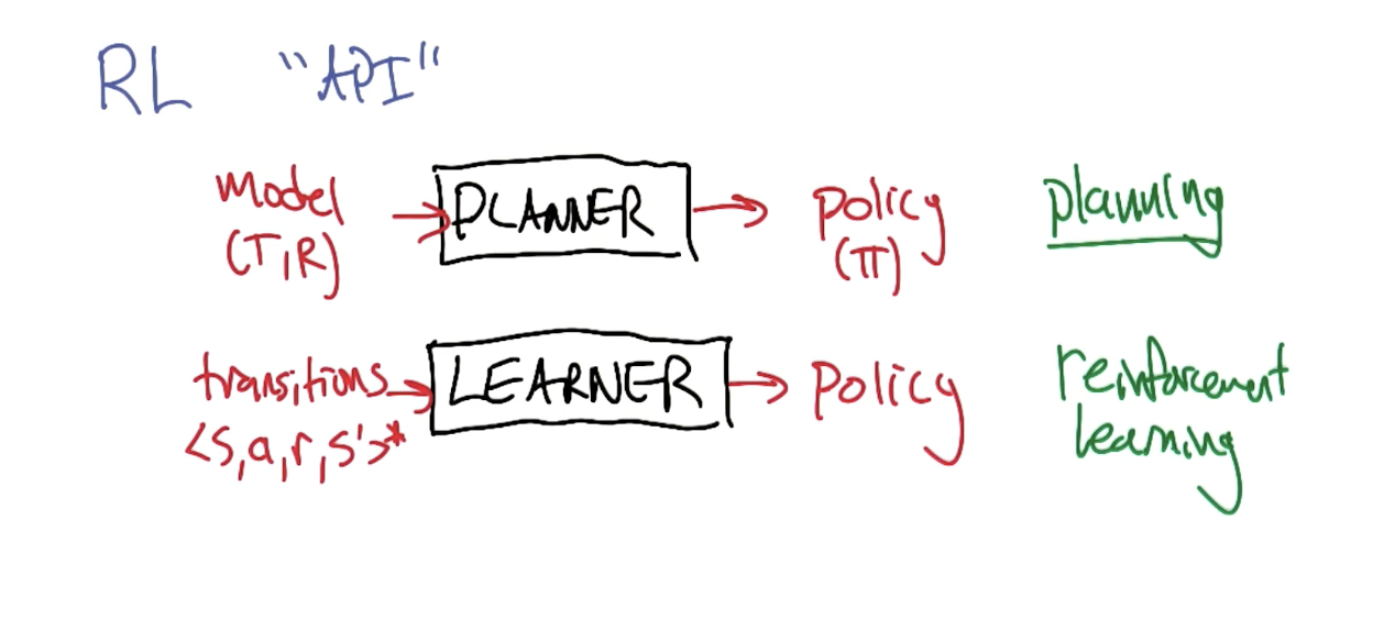
• Model-Based Planning: methods for solving MDPs, including Value Iteration and Policy Iteration. Require full specification of MDP components.

We ended the last module by discussing model-based methods for solving MDPs. However, in practice, we typically don’t know the true values for MDP components such as the state transition matrix or reward function.

Practical reinforcement learning algorithms learn from data, where data is composed of instances of the form $<s, a, r, s’>$. Although the input differs, the objective is still the same - we are interested in computing the optimal policy for our reinforcement learning problem represented via an MDP.

RL Algorithms

State-Action Value Function

Before discussing alternative approaches to solving MDPs, we introduce a new kind of value function. The State-Action Value Function (also called the Q-function) assigns value to the combination of state and action. It is a direct extension of the Bellman Equation.

\[Q(s, a) = R(s) + \gamma \sum_{s'} T(s, a, s') \max_{a'} Q(s', a')\]

Given an estimate for $Q(s, a)$, we can define state utility as $\max_a Q(s, a)$ and policy as $\arg \max_a Q(s, a)$.

Q-Learning

Q-Learning uses instances of transitions $<s, a, r, s’>$ to directly estimate the Q-function. The update rule is at the core of Q-Learning.

\[\hat{Q}(s, a) \leftarrow^{\alpha} r + \gamma \max_{a'} \hat{Q}(s', a')\]

Alpha represents the learning rate, which controls how quickly we update our estimate of $Q$.

\[Q_{t+1} \leftarrow (1 - \alpha) Q_t + \alpha \left(r + \gamma \max_{a'} Q_t(s', a')\right)\]

To be more accurate, Q-Learning is actually a class of RL algorithms which compute the optimal policy by estimating the Q-function. Variants of Q-Learning center on the following components.

• How do we initialize $\hat{Q}$?
• How do we decay $\alpha_t$?
• How do we select actions?

Action Selection

Given a Q-Learning algorithm, we might propose selecting actions by utilizing our current estimate of the Q-function. This is known as greedy selection.

\[\pi(s) = \arg \max_a \hat{Q}(s, a)\]

However, this strategy can lead us to become stuck in local minima, where we only explore a subset of the actions that the Q-function currently thinks is “good” (relative to other actions).

In the context of reinforcement learning, Exploration vs. Exploitation refers to the tradeoff between random action selection (exploration) and utilization of the current Q-function for action selection (exploitation). More specifically, epsilon-greedy exploration selects actions in a stochastic manner.

\[\Pr(a) = \begin{cases} a \sim \text{Uniform} & \epsilon \\ \arg \max_a \hat{Q}(s, a) & 1 - \epsilon \end{cases}\]

---

(all images obtained from Georgia Tech ML course materials)