ML M18: Game Theory (Part 1)

What is Game Theory?

Definition

According to Wikipedia, Game Theory is the study of mathematical models of strategic interactions. Game theory is primarily concerned with deriving optimal strategies for competitive situations involving two or more agents. We can concisely summarize game theory as the mathematics of conflict.

In previous lessons, we’ve explored reinforcement learning (RL) from the context of a single agent. The primary difference between standard RL and game theory is the number of agents. Game theory is concerned with the analysis of competitive situations, implying that we must have at least two interacting agents as part of the problem definition.

Example 1: Simple Game Tree

Consider a very simple example of game theory. Our problem is represented by the following game tree, which is a graphical structure enumerating all possible game states and decisions.

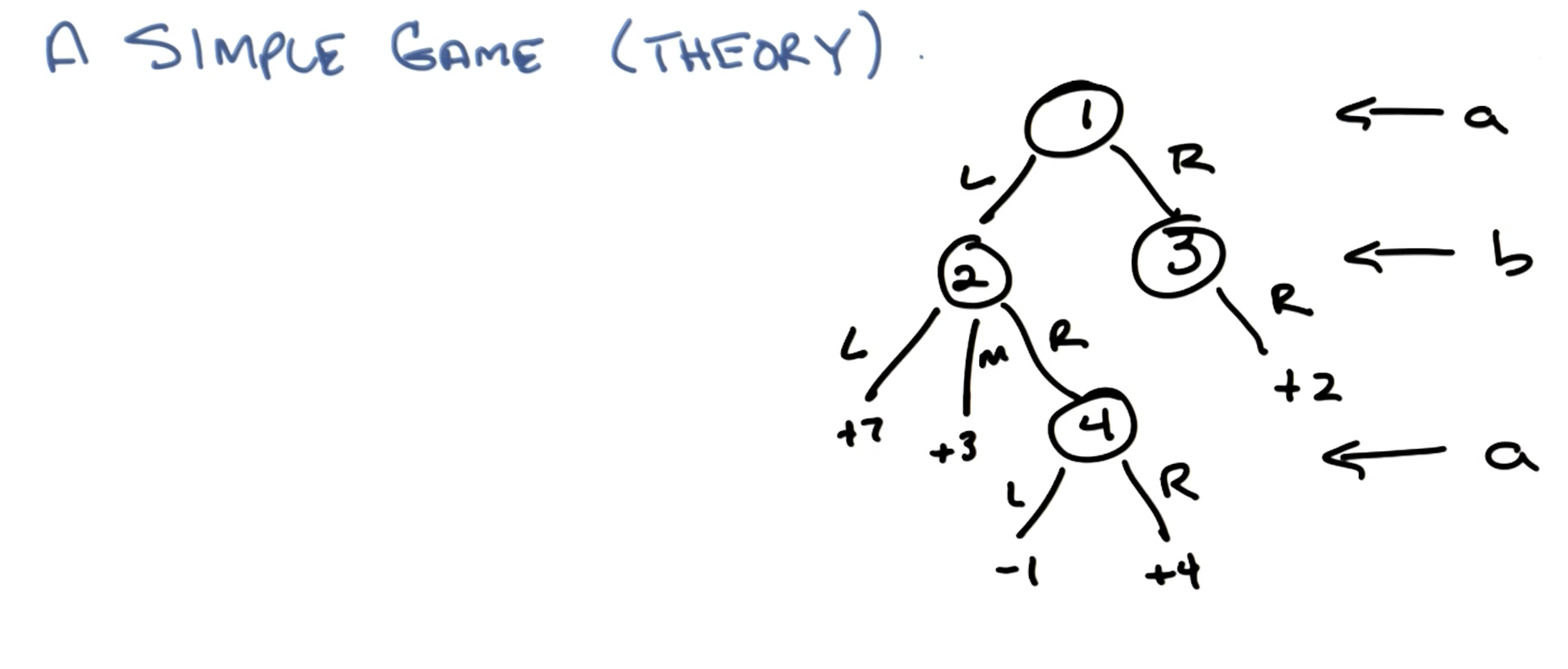
This is a two-player zero-sum finite deterministic game of perfect information. Let’s break down these characteristics a bit further:

• Two-Player: two agents interacting as part of the game.
• Zero-Sum: one agent’s reward is exactly balanced by the other agent’s loss.
• Finite: game is guaranteed to end after a finite number of moves.
• Deterministic: transitions have no element of randomness / stochasticity.
• Perfect Information: each agent has complete access to information (game states) throughout the entirety of the game.

A Strategy is analogous to a policy, but is specific to one agent in the game. In other words, a strategy maps all possible game states to actions for a given agent. In the above example, how many strategies are possible for each of the agents?

• Agent A: $2 \times 2 = 4$.
  • Two choices at Node $1$, two choices at Node $4$.
  • In order to be a strategy, we must have full specification over all states. This means even in the case where Agent A selects $R$ as the first move, we should still specify their move at Node $4$.
• Agent B: $3 \times 1 = 3$.
  • Three choices at Node $2$, one choice at Node $3$.

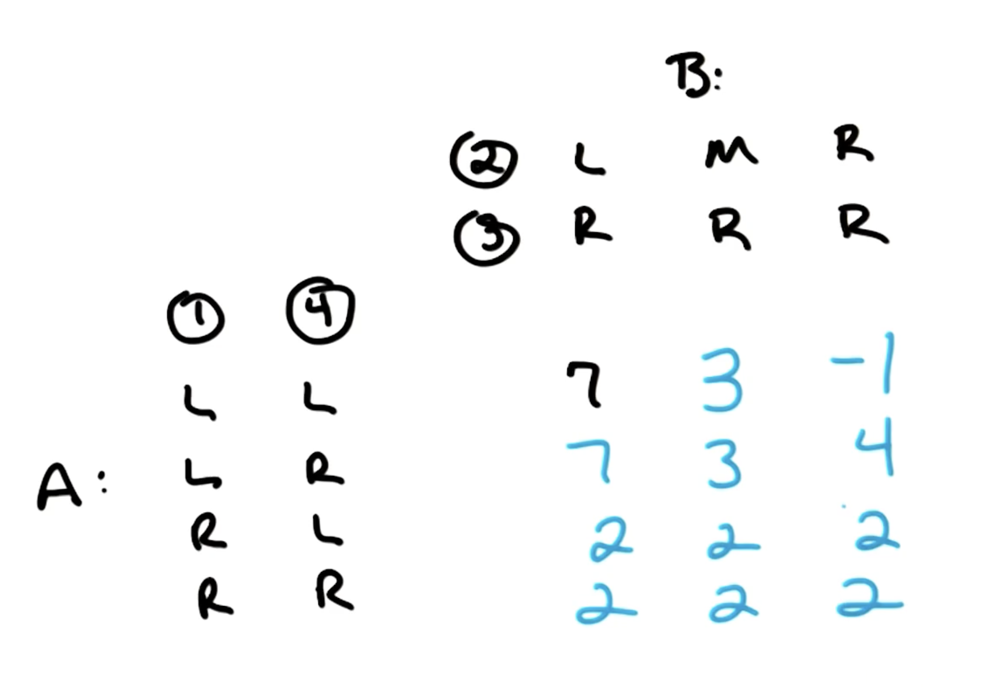
A game matrix (also known as payoff matrix) for a two-player game is a table with rows corresponding to strategies for one agent, and columns denoting strategies for the other agent. Cells of the matrix represent outcome values (rewards, payoff) associated with a particular combination of strategies.

Example 2: Mini-Poker

Consider another example which relaxes one of our previous constraints. We define Mini-Poker according to the following rules:

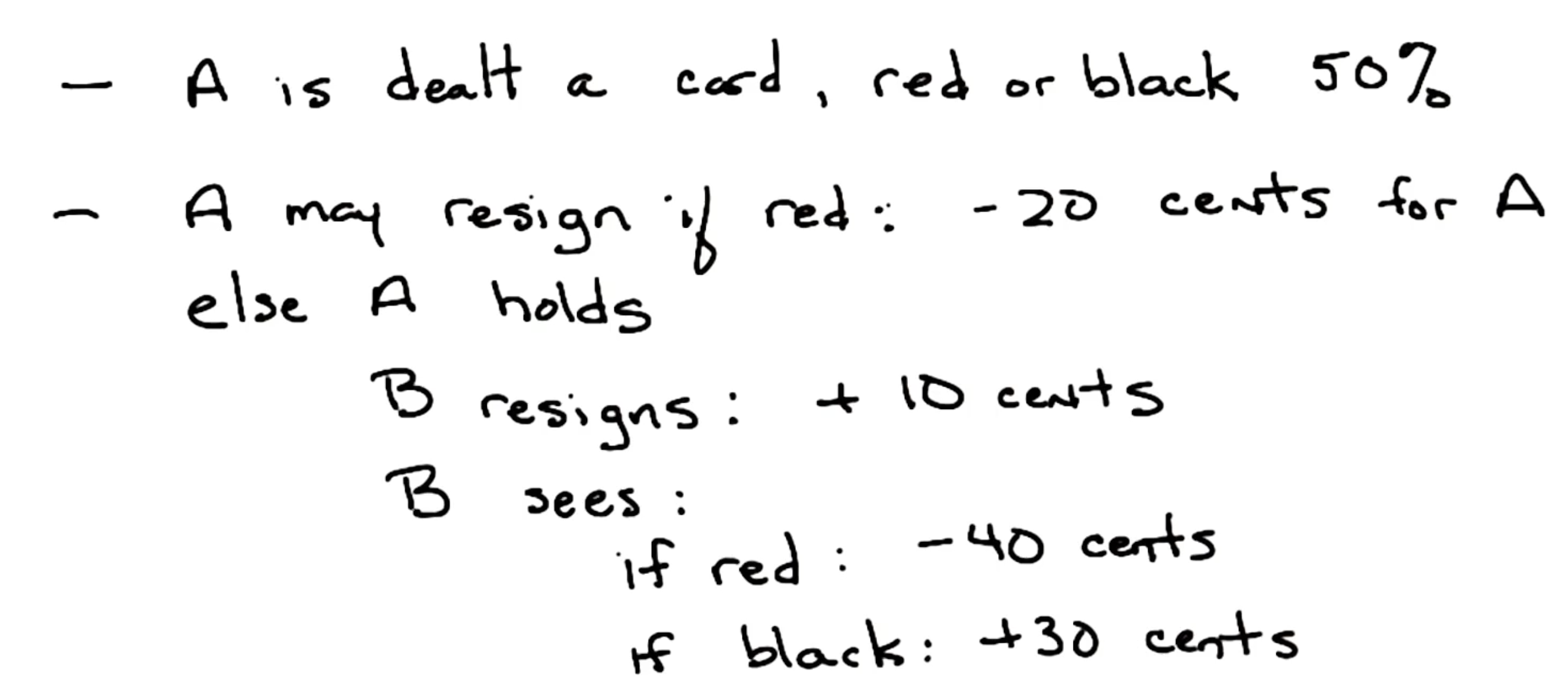
This implies mini-poker is a two-player, zero-sum, non-deterministic game of hidden information. Similar to the previous example, we can represent this game via a game tree.

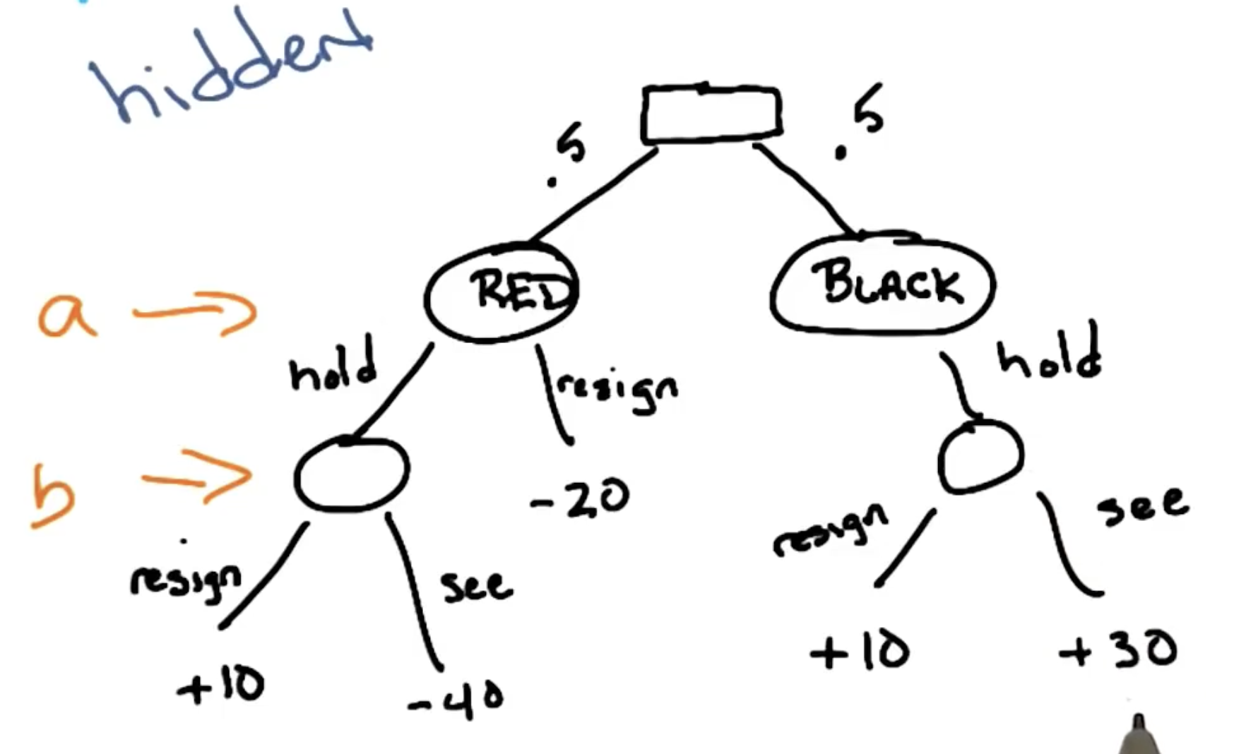
In the previous example, Agent B knew which branch of the game tree they were in (since the game involved perfect information). As part of mini-poker, Agent B does not have access to this information!

Example 3: Prisoner’s Dilemma

Finally, let’s present an example which relaxes our constraints even further. As part of the classic Prisoner’s Dilemma game, two prisoners are asked to snitch on each other with the following action / reward scheme.

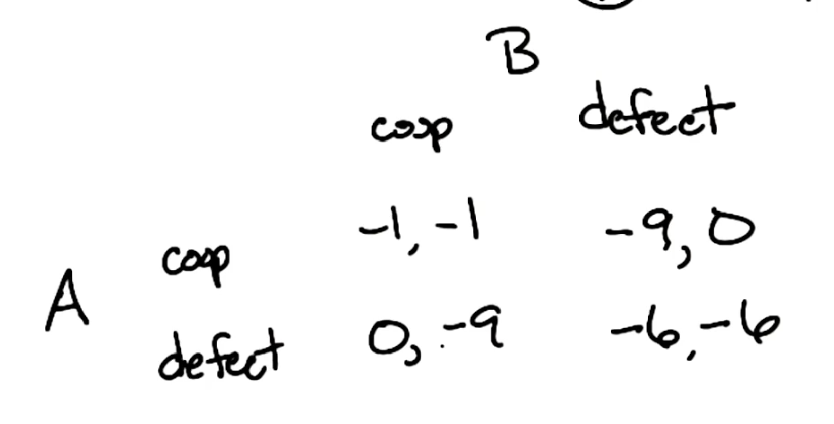
This game represents a two-player, non-zero-sum, non-deterministic game of hidden information.

Game Theory Algorithms + Concepts

Minimax

The Minimax algorithm is used to derive optimal strategies for a two-player zero-sum game. More specifically, minimax assumes one agent is playing to maximize their own score, while the other agent is playing to minimize this same score.

Computationally, minimax is a recursive depth-first search algorithm. Given a game tree, with leaves representing final game states and scores assigned to each leaf, minimax selects the action corresponding to maximum reward at Agent A’s turns, and the action corresponding to minimum reward at Agent B’s turns. This selection process begins at leaf nodes and proceeds upwards through the game tree.

As part of a two-player, zero-sum, deterministic game of perfect information, there always exists an optimal pure strategy for each player. This is known as Von Neumann’s Theorem.

Mixed Strategies

In our first example involving the simple game tree, we assumed pure strategies - strategies where the agent makes a single deterministic choice for every trial of the game. In contrast, mixed strategies introduce stochasticity into action selection by setting a distribution over strategies.

Nash Equilibrium

The Nash Equilibrium of a $n$-player game refers to the set of optimal strategies such that no single player within the set would change their strategy given the choice. Nash Equilibrium applies in the case of both pure and mixed strategies.

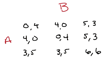
\[\forall_i s^{*}_i = \arg \max_{s_i} \text{utility}(s^{*}_1, \ldots, s_i, \ldots, s^{*}_n)\]

In the case of the Prisoner’s Dilemma, the Nash Equilibrium is the case in which both prisoners defect. The Nash Equilibrium in the following quiz is $(A: \text{Option} ~ 3, ~ B: \text{Option} ~ 3)$.

Three fundamental theorems stem from the definition of Nash Equilibrium.

• In the $n$-player pure strategy game, if elimination of strictly dominated strategies eliminates all but one combination, that combination is the unique Nash Equilibrium.
  • Strictly Dominated: action that is always worse than another action, regardless of the opponent’s choice.
• Any Nash Equilibrium will survive elimination of strictly dominated strategies.
• If $n$ is finite and the set of strategies is finite, there exists at least one Nash Equilibrium.

Furthermore, for any game repeated $n$ times, the Nash Equilibrium is the same for each game in the sequence ($n$-repeated N.E.).

---

(all images obtained from Georgia Tech ML course materials)