ML M19: Game Theory (Part 2)

Iterated Prisoner’s Dilemma

Review

In the previous lesson, we introduced the following concepts.

• Game Theory: mathematics of conflict. Concerned with the study of mathematical models and reward maximization in the context of a multi-agent world.
• Prisoner’s Dilemma: classic game theory example involving two prisoners who are asked to snitch on one another in exchange for reduced sentencing.
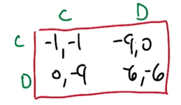
  • See below for the game (payoff) matrix summarizing the prisoner’s dilemma. Rows represent strategies for Prisoner A, and columns strategies for Prisoner B.
  • According to the game matrix, the optimal strategy for each prisoner is to defect (D) as opposed to cooperate (C) with one another.

Furthermore, we defined an iterated prisoner’s dilemma as a sequence of $n$ trials of the prisoner’s dilemma. Optimal strategies for the (finite + certain length) iterated version are the same as for a single trial. This is because the final game may be treated like a single game, and via proof by induction, each of the prior games may be treated as a single game given the subsequent game’s results are fixed.

Game Sequences with Uncertainty

What if instead of a fixed number of iterations $n$, there was uncertainty regarding the number of prisoner’s dilemma trials? First, we should define a mathematical representation for this scenario.

LOOP UNTIL BREAK

1. Run trial of prisoner’s dilemma.
2. Continue with probability $\gamma$, and break with probability $1 - \gamma$.

The expected number of trials $n$ is therefore $\frac{1}{1 - \gamma}$. Tit-for-Tat is a famous iterated prisoner’s dilemma (IPD) strategy which involves the following:

1. Cooperate on first trial.
2. Copy opponent’s previous move thereafter.

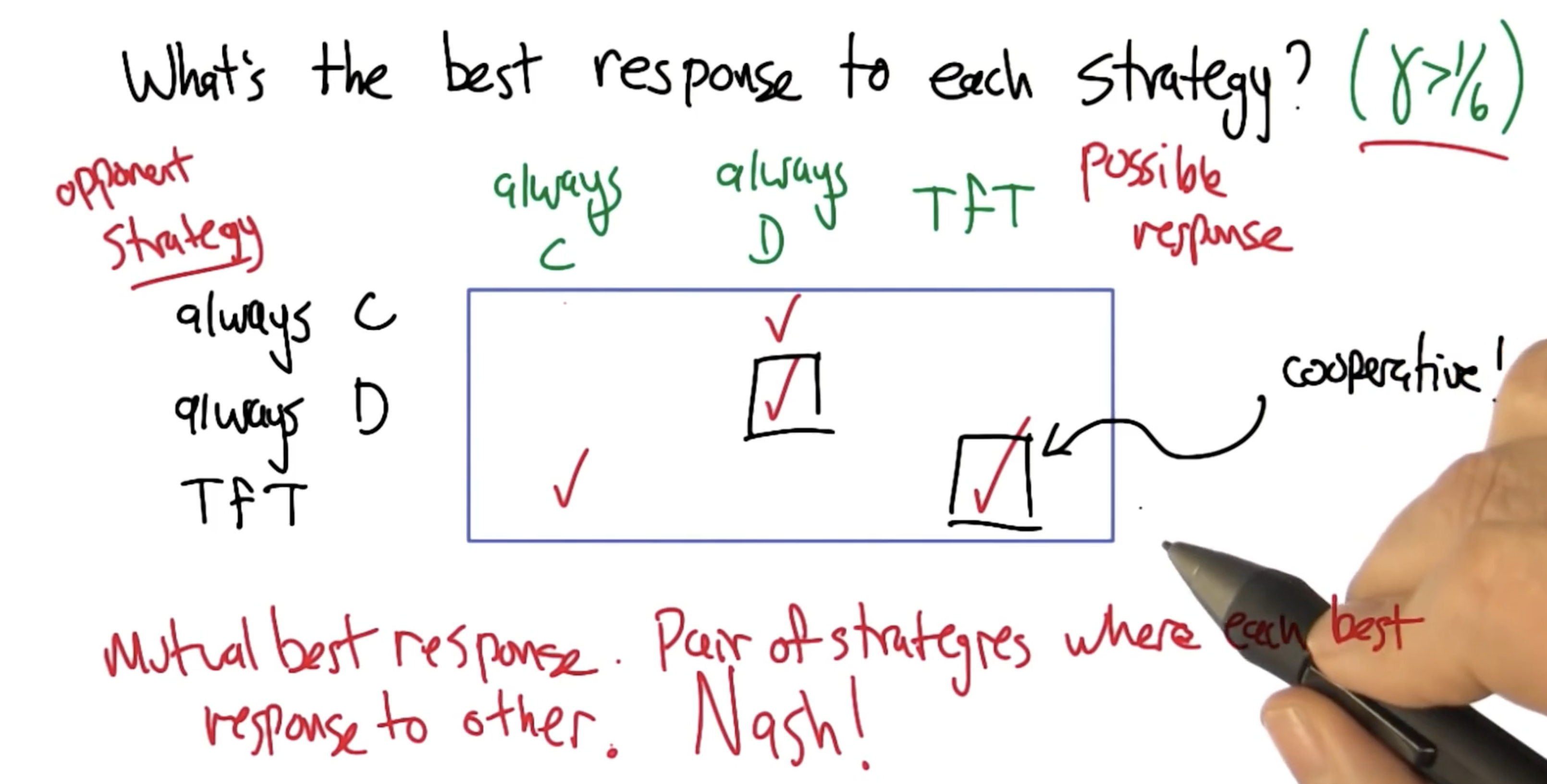
Interestingly, the optimal strategy in the iterated prisoner’s dilemma (IPD) is not to always defect. Instead, the strategy depends on 1) the specific value of termination $\gamma$, and 2) the opponent’s strategy.

Game Theory Concepts

Minmax Profile

In the context of game theory, a Minmax Profile defines a set of payoffs representing the reward which can be achieved by each player defending itself from a malicious strategy. Put more simply, the minmax profile represents the best result for each player under the worst-case scenario.

Folk Theorem

The key idea behind the Folk Theorem of game theory is that in repeated games, the possibility of retaliation opens the door for cooperation.

Any feasible payoff profile that strictly dominates the minmax profile can be realized as a Nash Equilibrium payoff profile, given a sufficiently large discount factor.

We define a feasible payoff profile as a valid payoff structure resulting from some combination of strategies across repeated iterations of the game. Given this definition, the Folk Theorem is making two key assertions:

• If a feasible payoff profile is better than the minmax (meaning individual player payoffs are each better as opposed to their minmax counterparts), it would be better for the players to cooperate as opposed to choosing the minmax. In other words, players would be punished (held to their minmax payoff) for defecting, thereby making cooperation sustainable.
• There may be multiple Nash Equilibria within a game. In fact, there may be an infinite number of possible Nash Equilibria in repeated games.

In general, any “Folk Theorem” refers to a principle in mathematics which has established status but is not published in its complete form.

Grim Trigger

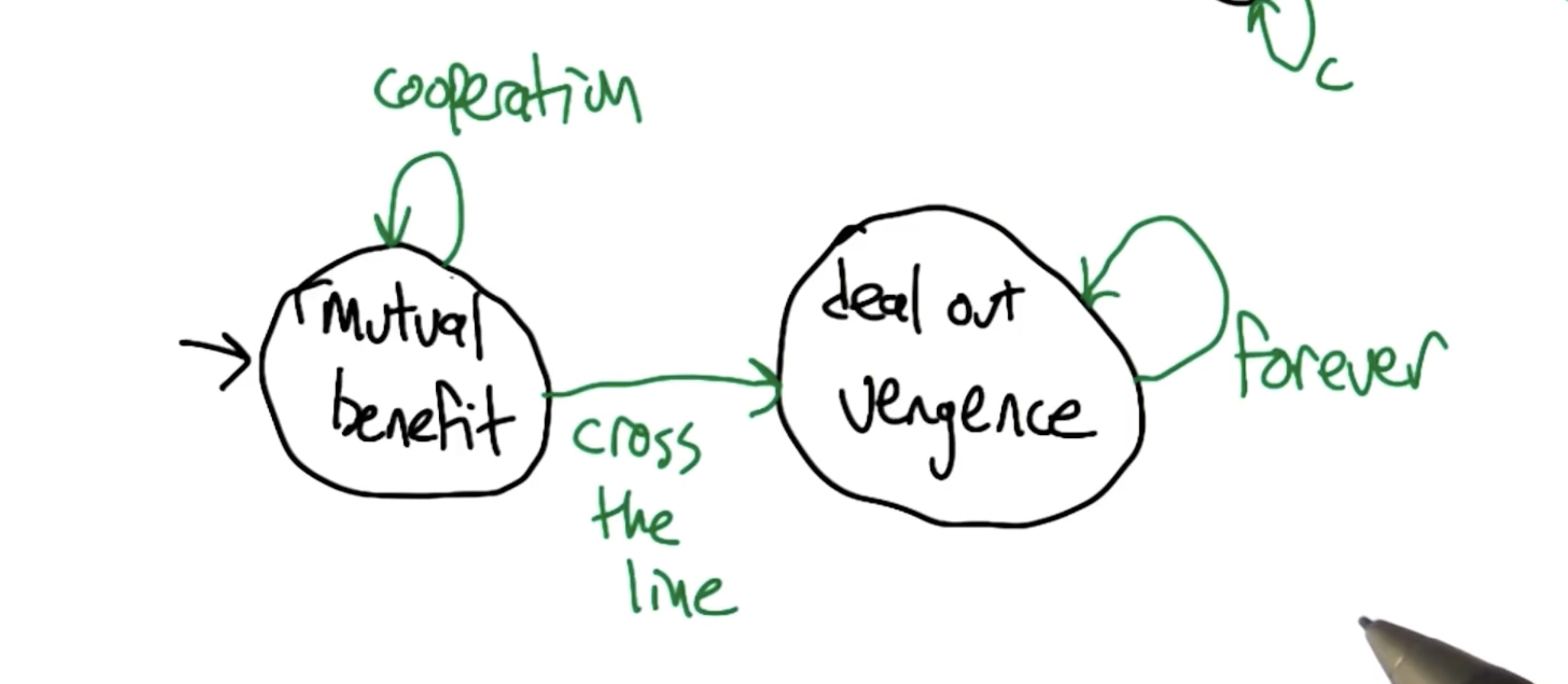
Grim trigger is a type of strategy which involves cooperation until defection. If any player decides to defect from cooperation, the other player will choose the more punishing option for the remaining iterations.

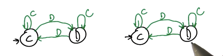
Pavlov

Pavlov’s Strategy seeks to take advantage of the opponent for as long as possible. Given that the opponent is cooperating, Pavlov’s strategy will also cooperate. At the first sign of defect, we switch to defecting; even if the opponent begins to cooperate, we will continue to defect until our opponent also defects. At that point, we switch back to cooperating.

Pavlov vs. Pavlov is considered a Nash Equilibrium since both players will start off cooperating, and always cooperate thereafter.

Reinforcement Learning

Stochastic Games and Multi-Agent RL

Stochastic Games are the extension of Markov Decision Processes (MDP) to the multi-agent setting. This concept was introduced by Lloyd Shapley in 1953. Similar to MDPs, stochastic games are defined by a series of components:

• States $s \in S$
• Actions for each Player $a \in A_1(s)$, $b \in $A_2(s)$
• State Transition Matrix $T(s, (a, b), s’)$
• Rewards for each Player $R_1(s, (a, b))$, $R_2(s, (a, b))$
• Discount Factor $\gamma$

Note there are a few key differences between stochastic games and MDPs. First, the state transition matrix is defined in terms of the set of player actions taken at some iteration. Additionally, we must define a separate reward function for each of the players.

Zero-Sum Stochastic Games

In the case of zero-sum stochastic games, the reward for one player is directly opposite the reward for the other. \(R_1 = -R_2 ~~ \therefore ~~ R_1 + R_2 = 0\)We can apply the Bellman Equation to zero-sum stochastic games by making a few tweaks to the original version. Note that the version below is NOT fully correct for one key reason.

\[Q_i^{*}(s, (a, b)) = R_i(s, (a, b)) + \gamma \sum_{s'}T(s, (a, b), s') \max_{a', b'} Q_i^{*}(s', (a', b'))\]

• We are evaluating $Q$ relative to Player $i$ - in other words, quality for the same set of state-action pairs will be different for different players.
• By taking the $\max$ of $Q_i$ over actions $a$ and $b$, we are implying that both players will select actions to maximize $Q_i$. This is optimistically delusional - given you are Player $A$, your opponent Player $B$ will not select their actions to maximize your own reward $Q_A$!

Recall that minimax selects actions for a two-player zero-sum game by assuming one player will choose actions to maximize their own score, while the other will choose actions to minimize that player’s score. We can apply this concept as part of our definition for $Q$.

\[Q_i^{*}(s, (a, b)) = R_i(s, (a, b)) + \gamma \sum_{s'}T(s, (a, b), s') \text{minimax}_{a', b'} Q_i^{*}(s', (a', b'))\]

Given our definition of $Q$, we can now define Q-Learning in the context of stochastic games! This algorithm is called minimax-Q.

\[Q_i(s, (a, b)) \leftarrow^{\alpha} r_i + \gamma \text{minimax}_{a', b'} Q_i(s', (a', b'))\]

General Sum Stochastic Games

Minimax is a Nash Equilibrium in two-player, zero-sum games. Unfortunately, minimax only applies to zero-sum games - this is because minimax assumes the opponent is playing to minimize our own score, which results from the opponent’s score being a function of our own score.

In game theory, General Sum games refer to any situations where players’ payoffs aren’t fixed to sum to zero (or any constant). This implies there are scenarios where both players may “win” or “lose”, depending on the definitions of these conditions within our world.

In the case of general sum games, we should alter our $Q$ equation to define action selection based on whatever Nash Equilibrium applies to the game, instead of using minimax as in the case of two-player zero-sum games. This algorithm is known as Nash-Q.

\[Q^{*}_i \leftarrow^{\alpha} r_i + \gamma T(s, (a, b), s') \text{Nash}_{a', b'} Q^{*}_i(s', (a', b'))\]

Unfortunately, many characteristics of Q-Learning (and minimax-Q) do NOT apply in the case of Nash-Q.

• Value iteration doesn’t work.
• Nash-Q is not guaranteed to converge.
• There is no unique solution to $Q^{*}$.
• Policies cannot be computed independently.

There are alternative methods for solving general sum games, but this is outside the scope of the current course.

---

(all images obtained from Georgia Tech ML course materials)