ML M2: Decision Trees

Supervised Learning

Definition

Supervised Learning refers to function approximation - given a labeled set of tabular data consisting of features $X$ and labels $y$, we are interested in mapping from input features to output labels.

\[f : X \rightarrow y\]

There are two primary types of supervised learning:

• Classification: discrete output label; may be binary or multiclass depending on output dimensionality.
• Regression: continuous output label; $y \in \mathbb{R}$.

Vocabulary

From a theoretical standpoint, we should define some foundational terminology which will appear frequently over the supervised learning lectures:

• Instance: vector of realized attributes (random variables) defining the input space. An instance is a single realization of a series of random variables. $\mathbf{x} = \begin{bmatrix} x_1 & \ldots & x_p \end{bmatrix}$
• Concept: functional mapping between inputs and outputs. The target concept is the true functional representation which we are interested in finding!
• Hypothesis Space: set of all possible concepts for the given problem. We restrict our hypothesis space by selecting a certain modeling approach (e.g., binary classification with decision trees restricts our set of possible representations).
• Training Set: data used to train the model; each instance must have an input $x$ paired with its respective correct output label $y$.
• Test Set: data used to evaluate the model, following the same structure as the training set; important for estimating model generalization to unseen instances.
  • Data leakage occurs when information from the training set contaminates the test set, and therefore skews our estimation of model generalizability.

Decision Trees for Classification

General Approach

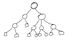
A Decision Tree is a nonparametric supervised learning algorithm that uses sequential splitting to make predictions. Each decision node (circle) splits data depending on the value of some attribute. Leaf nodes are final destinations in the tree where predictions are generated.

Learning in the context of decision trees refers to selecting attributes and split values for decision nodes. The best split should minimize post-split node impurity - in the case of classification, this value may be approximated by the Gini Index or Entropy.

\[\text{Gini Index}: ~~~ I_G = 1 - \sum_j^k p_j^2 ~~~~ k = \text{n classes}\] \[\text{Entropy}: ~~~ I_H = - \sum_j^k p_j \log_2 p_j\]

Put differently, the best split should maximize information gain - weighted reduction in expected entropy as a result of the split.

\[\text{Information Gain}: ~~~ G(S, A) = \text{Entropy}(S) - \sum_v \frac{|S_v|}{|S|} \text{Entropy}(S_v)\]

Decision tree algorithms typically proceed by greedily selecting the best possible split until reaching some terminal condition.

ID3 Algorithm

ID3 is a specific algorithm for fitting decision trees that implements the above concepts.

Loop over iterations:
    Loop over leaves:
        1. Identify best attribute $A$ according to information gain.
        2. Assign $A$ as decision attribute for node and sort training instances to leaves.
        3. Check terminal condition (perfect classification).

As with any machine learning algorithm, ID3 has certain inductive biases which influence the search for the optimal concept.

• Restriction Bias: bias introduced as a result of the available hypothesis space. ID3 only considers decision trees, so we will not obtain any other type of concept!
• Preference Bias: indicates which hypotheses from the available set are preferred. ID3 prefers concept trees which 1) model the data correctly, 2) contain better splits at the top, and 3) are shorter in depth.

Other Considerations

Splitting is relatively straightforward in the case of a binary attribute. However, what if we have a continuous attribute? We can define splits as ranges (ex: age $\geq$ 30), and iterate over all unique values for the attribute in the training set as candidate split values.

We defined the terminal condition for ID3 as perfect classification. What if we have noise in our data, preventing perfect classification and causing an infinite loop? We can refine our terminal condition to stop after reaching a maximum depth instead.

Finally, overfitting is an issue with any machine learning algorithm. We can introduce modifications into the ID3 algorithm to mitigate overfitting. For example, early stopping will terminate training after validation error fails to decrease over some number of rounds. Pruning is another approach which removes terminal decision nodes based on validation error after the decision tree has been fit.

---

(all images obtained from Georgia Tech ML course materials)