ML M3: Regression
Module 3 of CS 7641 - Machine Learning @ Georgia Tech. Lesson 2 of Supervised Learning Series.
Regression
Recall that supervised learning is the subfield of machine learning concerned with function approximation. Given input features $\mathbf{X}$ and output feature(s) $\mathbf{y}$, any supervised learning algorithm estimates the functional mapping from $\mathbf{X}$ to $\mathbf{y}$.
\[f: \mathbf{X} \rightarrow \mathbf{y}\]Regression is supervised learning applied to a continuous output variable $\mathbf{y} \in \mathbb{R}$. Regression is a general category of supervised learning algorithms, not to be confused with the topic of the next section.
Linear Regression
Linear Regression is a specific type of regression method which uses a linear model to represent the relationship between inputs and output.
\[\mathbf{\hat{y}} = \mathbf{X}\mathbf{w} ~~~~ \mathbf{X} \in \mathbb{R}^{n \times p}, ~ \mathbf{w} \in \mathbb{R}^{p}\]The model is fit by determining the optimal values for the parameter vector $\mathbf{w}$. Okay, but how? The normal equation directly solves this optimization problem using calculus. We define an objective function to evaluate the quality of our fit - mean squared error - and optimize our parameter values relative to this function.
Derivation of Normal Equation
Let’s quickly derive the normal equation via ordinary least squares. We start with our objective function, which is simply the definition of mean squared error. For any given instance $i$, $\hat{y_i}$ represents the associated model prediction and $y$ its ground truth label.
\[L(\mathbf{w}) = \frac{1}{n} \sum_i (y_i - \hat{y}_i)^2 \tag{1}\]We can convert this objective function to its linear algebra equivalent, and drop the $\frac{1}{n}$ term since it has no effect on optimization.
\[L(\mathbf{w}) = (\mathbf{y} - \mathbf{\hat{y}})^T(\mathbf{y} - \mathbf{\hat{y}}) \tag{2}\]After some substitution and expanding, we have an equation which is ready for optimization.
\[L(\mathbf{w}) = (\mathbf{y} - \mathbf{Xw})^T(\mathbf{y} - \mathbf{Xw}) \tag{3}\] \[L(\mathbf{w}) = \mathbf{y}^T\mathbf{y} - \mathbf{y}^T\mathbf{Xw} - \mathbf{w}^T\mathbf{X}^T\mathbf{y} + \mathbf{w}^T\mathbf{X}^T\mathbf{Xw} \tag{4}\] \[L(\mathbf{w}) = \mathbf{y}^T\mathbf{y} - 2\mathbf{w}^T\mathbf{X}^T\mathbf{y} + \mathbf{w}^T\mathbf{X}^T\mathbf{Xw} \tag{5}\]This function can be optimized by differentiating w.r.t. our parameter vector $\mathbf{w}$. Recall that any location with zero first derivative is a critical point. Furthermore, our equation is convex, which implies any local optimum is also the global optimum. We can therefore set our first derivative equal to zero to solve for the optimal parameter vector.
\[\frac{\partial}{\partial{\mathbf{w}}}L = \frac{\partial}{\partial{\mathbf{w}}} \left [ \mathbf{y}^T\mathbf{y} - 2\mathbf{w}^T\mathbf{X}^T\mathbf{y} + \mathbf{w}^T\mathbf{X}^T\mathbf{Xw} \right ] \tag{6}\] \[0 = -2\mathbf{X}^T\mathbf{y} + 2\mathbf{X}^T\mathbf{Xw} \tag{7}\] \[\mathbf{w} = (\mathbf{X}^T\mathbf{X})^{-1} \mathbf{X}^T \mathbf{y} \tag{8}\]Polynomial Regression
The linear model is considered linear with respect to its parameters - $y$ is a linear combination of the weights (where linearity may only involve addition or scaling). However, this does not mean we are limited to a purely linear representation. By introducing higher-order features into the input matrix $\mathbf{X}$, we still have the same formula as before!
\[\mathbf{x}_{\text{old}} = \begin{bmatrix} x_1 &\ldots & x_p \end{bmatrix}\] \[\mathbf{x}_{\text{new}} = \begin{bmatrix} x_1 & x_1^2 & \ldots & x_p & x_p^2 \end{bmatrix}\]For example, a second-order polynomial involving a single input feature $x$ might look as follows:
\[\mathbf{\hat{y}} = w_1x_1 + w_2x_1^2 + b\]More generally, Polynomial Regression utilizes the framework of linear regression, but introduces polynomial features into the input matrix to enable non-linear representation.
We do have one issue here - how do we select the polynomial order for our problem? Higher-order polynomials will always fit training data better due to their increased variance. This does NOT mean we should default to the highest possible order.
Generalization
What is Cross Validation?
One of the most fundamental considerations in machine learning is Generalization, which refers to a model’s performance on unseen data. Training dataset performance does not properly represent generalization by definition - the model has seen this data during training, and has therefore been tweaked to fit these data points as closely as possible. Instead, we use a held-out test set to estimate model generalization.
Given a single dataset, how do we form our test set? We can perform a simple train-test split to randomly separate data into training and test partitions. Alternatively, K-Fold Cross Validation is a technique which divides a dataset into $k$ partitions. Then, each partition is used as a test set while the other $k-1$ partitions are used to train the model. Final model generalization is estimated as the average performance over test sets.
The primary benefit of using cross validation over a train-test split is to reduce the variance of our estimate. However, we typically use train-test splits in the context of very large data, and cross validation for smaller data. This is because cross validation is much more computationally demanding!
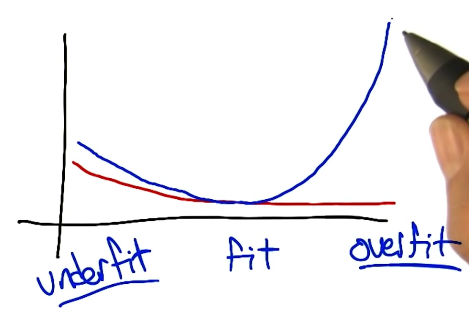
Bias-Variance Tradeoff
For any machine learning model, we have a tradeoff between two competing concepts:
- Variance: complexity (flexibility) of the model; representational power.
- Bias: assumptions of the model limiting representation.
Overfitting refers to the case where a model fits the training data well, but this performance does not transfer to the test set (overfitting exists on a gradient as opposed to being a simple 0/1 status). We can mitigate overfitting by limiting the variance of our model, but we should also ensure our model has sufficient representational power to capture the true concept.
Hyperparameter Tuning
Most machine learning algorithms have hyperparameters, which are any parameters set to define configurable portions of the model fitting process (as opposed to being directly learned from the data). For example, in the case of polynomial regression, order is a hyperparameter influencing the variance of the model!
To select the best hyperparameter for our problem, we perform hyperparameter tuning. This involves repeating the model training process on many candidate hyperparameter configurations, then selecting the best configuration to minimize generalization error. Note that in the case of hyperparameter tuning, we must actually split our dataset into three partitions:
- Training Set: used to train any given hyperparameter configuration.
- Validation Set: evaluates individual model performances; best hyperparameter configuration is selected based on performance here.
- Test Set: given a final model, estimates true generalization performance.
To revisit our polynomial regression example, we might select order as follows:
1) Fit multiple different models on the training dataset using different values for order (e.g., 1, 2, 3, 4). 2) Evaluate each model on the validation dataset. Identify the model which performs best, and use its value for order. 3) Re-fit the model on the combined training + validation set using the optimal value for order. 4) Evaluate final model performance on the test set to estimate model generalizability.
(all images obtained from Georgia Tech ML course materials)