ML M4: Neural Networks

What are Neural Networks?

Definition

An Artificial Neural Network is a machine learning model consisting of a series of interconnected mathematical transformations. Neural networks are inspired by the human brain / neurons, but they do not directly replicate any biological function.

Neural networks are organized as a series of layers, which represent mathematical transformations. Nodes within the previous layer are the operands of the transformation, whereas those in the current layer are the result. Additionally, neural networks have an input layer with nodes representing features, and an output layer generating final results. For example, consider the following neural network with two hidden layers and three nodes per hidden layer.

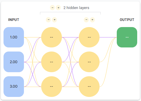
The mathematical representation for a neural network is relatively straightforward. Since we are applying sequential transformations, we can define our neural network as a series of nested functions applied to the original input. Consider the formula for the above example:

\[\textbf{X} \in \mathbb{R}^{n \times 3}, \mathbf{W_1} \in \mathbb{R}^{3 \times 3}, ~ \mathbf{W_2} \in \mathbb{R}^{3 \times 1}, ~\textbf{y} \in \mathbb{R}^{n \times 1}\] \[\mathbf{\hat{y}} = h_2(h_1(\mathbf{X})) ~~~~ h_1 = \sigma(\mathbf{XW_1}) ~~~~ h_2 = \sigma(\mathbf{H_1}\mathbf{W_2})\]

In most networks, each layer is the combination of a linear transformation followed by a non-linear activation function. The non-linear component enables neural networks to have extreme representational power; if the network were composed of sequential linear transformations alone, it would have the same representational capacity as a single linear transformation!

\[h_1(\mathbf{X}) = \mathbf{XW_1} ~~~~ h_2(\mathbf{H_1}) = \mathbf{H_1W_2} ~~~~ \rightarrow ~~~~ h_2(h_1(\mathbf{X})) = \mathbf{XW_1W_2} ~~~~ \mathbf{W_1W_2}\] \[\text{Let} ~ \mathbf{W_3} = \mathbf{W_1W_2} ~~~~ \rightarrow ~~~~h_2(h_1(\mathbf{X})) = \mathbf{XW_3}\]

Biases

Recall that restriction bias indicates the set of hypotheses a modeling class considers. Neural networks are not very restrictive due to their extreme representational power. In theory, a neural network should be able to represent any function given appropriate complexity (which results from # layers, # nodes, and non-linear activation types). The downside of this representational power is the high potential for overfitting.

Preference bias influences the types of hypotheses an algorithm will select based on its nature. Neural networks also have weak preference bias, mostly influenced by user-level specifications on the optimization approach. For example, methods such as random weight initialization to small values and regularization prefer simpler representations to more complex ones (Occam’s Razor!).

Perceptron

The simplest type of neural network is the Perceptron, which has a single layer consisting of a linear transformation followed by a non-linear thresholding operation. The perceptron was originally introduced by Frank Rosenblatt in 1957 at Cornell University.

\[y = \begin{cases} 1 & \text{if} ~~\Sigma w_ix_i - \theta > 0 \\ 0 & \text{otherwise} \end{cases}\]

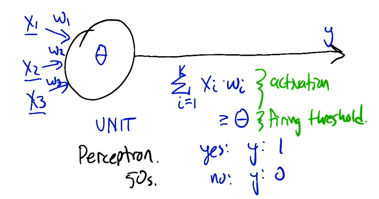
Given two binary inputs, a perceptron has the ability to represent basic logical functions including AND, OR, and NOT. However, at least two perceptron units in sequence are required to represent XOR. This is because AND, OR, and NOT are linearly separable whereas XOR is not.

Neural Network Training

Perceptron Training

The Perceptron Rule defines an optimization approach for a single perceptron unit. We iterate over the following update step until reaching perfect classification (in the case of linear separability).

\[w_j^{(1)} = w_j^{(0)} + \Delta w_j \tag{1}\] \[\Delta w_j = \eta (y - \hat{y})x_j \tag{2}\]

The learning rate $\eta$ limits the size of parameter value updates at any given step.

Gradient Descent

We cannot apply the perceptron rule to neural networks for multiple reasons:

• Most neural networks have multiple “perceptron unit” components (corresponding to layers).
• The intermediate outputs of layers - called activations - are not binary.
• Layers are not limited to a thresholding operation, but rather any differentiable non-linearity.

In the case of neural networks, we use Gradient Descent for weight optimization. Gradient descent calculates the gradient of the loss function w.r.t. weights; the gradient of any multivariable scalar-valued function is the vector of partial derivatives corresponding to each variable. Following gradient calculation, weights are updated by taking a step in the direction of the negative gradient.

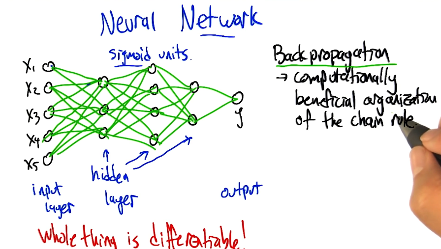
\[\nabla L(\mathbf{w}) = \begin{bmatrix} \frac{\partial{L}}{\partial{w_1}} & \ldots & \frac{\partial{L}}{\partial{w_p}} \end{bmatrix} \tag{1}\] \[\mathbf{w}^{(1)} = \mathbf{w}^{(0)} - \eta \nabla L(\mathbf{w}) \tag{2}\]

Okay, but how can we estimate the gradient for each of our weights? Backpropagation pushes the gradient of the loss backward through the network, calculating the gradient w.r.t. weights at each layer. This approach takes advantage of the chain rule of calculus.

\[\frac{\partial{L}}{\partial{w}} = \frac{\partial{L}}{\partial{h_2}} \times \frac{\partial{h_2}}{\partial{h_1}} \times \frac{\partial{h_1}}{\partial{w}}\]

In order to propagate the gradient backwards through the entire network, all intermediate components must be differentiable. Otherwise, we would have a “break” in the chain rule. This is why any non-linear activation function within a neural network must be differentiable!

Sigmoid

The Sigmoid function is a common choice for activation function, serving as a “soft” (differentiable) version of thresholding.

\[\sigma(z) = \frac{1}{1 + e^{-z}}\]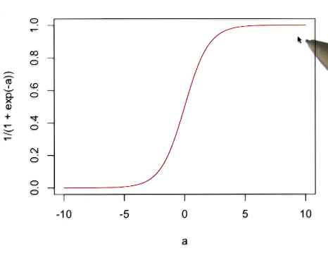

Not only is sigmoid differentiable; it also has an easy-to-work-with derivative!

\[\frac{\partial{\sigma}}{\partial{z}} = \sigma(z) \times (1 - \sigma(z))\]

---

(all images obtained from Google ML Crash Course and Georgia Tech ML course materials)