ML M5: Instance-Based Learning

What is Instance-Based Learning?

Instance-Based Learning refers to a class of supervised learning algorithms which directly reference instances in the training data to generate results. As opposed to learning a model-based representation using the training data, we directly compare new instances to the training data in order to generate a prediction. This approach works well when training data is very large and diverse.

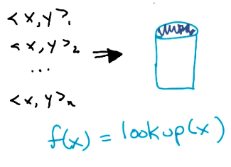
The simplest example of instance-based learning is a database lookup program. Given a set of training instances of the form $<x, y>$, we store instances in the database with keys corresponding to $x$ and values to $y$. Given a new instance $<x_n, y_n>$, we compare $x_n$ to our set of keys to generate the prediction $\hat{y}_n$.

There are certain pros and cons to this approach:

• PROS:
  • Not introducing any assumptions / biases via some model-based representation.
  • The approach is relatively fast compared to learning for other algorithms.
• CONS:
  • Models the training data exactly, which might imply overfitting.
  • Generalization is nonexistent - what happens if we have a new key $x_n$ that isn’t currently in the database?

Instead of our simple database lookup example, we will introduce a better defined instance-based learning algorithm in the following section.

K-Nearest Neighbors

Definition + Algorithm

The K-Nearest Neighbors (KNN) algorithm is similar to database lookup, but relies on the notion of similarity between instances to make predictions. Given a new instance $x_n$, we calculate the pairwise similarity between the new instance and each instance in our training dataset. Then, the $k$ most similar training instances inform the final prediction.

GIVEN:

• Training Data $D = \begin{Bmatrix} x_i & y_i \end{Bmatrix}$
• Query Point $q$
• Distance Metric $d(q, x)$
• Number of Neighbors $k$

NN = $\begin{Bmatrix} i: ~~ d(q, x_i) ~~ k ~ \text{smallest} \end{Bmatrix}$

In the case of classification, KNN predicts the mode of the most similar neighbors. For regression, KNN predicts the mean.

Hyperparameter Tuning

As with other machine learning algorithms, KNN has a number of Hyperparameters which must be optimized specific to the task at hand:

• Distance Metric: we can choose one of many functions to represent pairwise similarity. The most common choice is Euclidean Distance, but other options such as Manhattan Distance are also reasonable.
• Number of Neighbors $k$: the number of neighbors we use for predictions is perhaps the most important hyperparameter of the algorithm!

In order to perform hyperparameter tuning, we should use either a train-test split or cross validation to train our various hyperparameter configurations on the training partition(s), then optimize over performance on the validation (test) set.

Complexity

Let’s compare the time and space complexity of algorithm training and inference. Assume we are given training data as a set of $n$ sorted data points with only a single feature.

ALGORITHM		TIME COMPLEXITY	SPACE COMPLEXITY
1-NN	Learning	1	n
	Inference	log(n)	1
K-NN	Learning	1	n
	Inference	log(n) + k	1
Linear Regression	Learning	n	1
	Inference	1	1

Biases

Recall that preference bias describes an algorithm’s reasoning for selecting one hypothesis over another. In the context of KNN, there are three main factors which influence preference bias:

• Locality $\rightarrow$ similar points are closer in space (i.e., distance is a good representation of similarity).
• Smoothness $\rightarrow$ voting / averaging over neighbors is the appropriate method for prediction.
• Equal Feature Importance $\rightarrow$ distance is combined over all features in an equal fashion.

Miscellaneous Points on ML

The Curse of Dimensionality is a problem shared across supervised learning algorithms highlighting issues associated with high-dimensional data.

As the number of features or dimensions grows, the amount of data we need to generalize accurately grows exponentially.

Consider the following example:

• We are given a training dataset containing a single integer feature with domain of $\begin{bmatrix} 1 & 10 \end{bmatrix}$ and two instances: $x_1 = 1$ and $x_2 = 5$. Our training data occupies $\frac{1}{5}$ of the input space, since there are 10 possible inputs.
• We decide to add another integer feature to the training dataset, also with domain $\begin{bmatrix} 1 & 10 \end{bmatrix}$. Our instances are now $x_1 = \begin{bmatrix} 1 & 1 \end{bmatrix}$ and $x_2 = \begin{bmatrix} 5 & 5 \end{bmatrix}$. Now, our training data occupies $\frac{1}{50}$ of the input space - we would need 18 more different instances to cover the same portion of the input space as in the case of a single feature!

The more features we add to the problem, the more data we require to adequately represent the input space.

---

(all images obtained from Georgia Tech ML course materials)