ML M6: Ensemble Learning

What is Ensemble Learning?

Definition

Ensemble Learning refers to a class of supervised learning algorithms which relies on a collection of models (as opposed to a single model) to make predictions. The core idea behind ensemble learning is that a collection of simpler models may have better generalization compared to a single model with better fit to the training data.

Where does the notion of “simpler” come into play? Each model within an ensemble learns over a subset of the data, forming a simple concept. The ensemble then combines simple concepts into a more complex hybrid concept. Why is simpler better? Ensemble learning takes an approach loosely similar to cross validation - we learn over multiple subsets of the data, holding some portion out in each case. Each individual model will be somewhat noisy, but the final model averages out this noise to produce a smoother estimate.

More formally, we define a “simple model” as a weak learner, which must do at least better than random chance on the supervised learning problem.

\[\text{WEAK LEARNER}: ~~~\forall_\mathbb{D} ~~\Pr_{\mathbb{D}} [.] \leq \frac{1}{2} - \epsilon\]

Ensemble Learning Approaches

Bagging

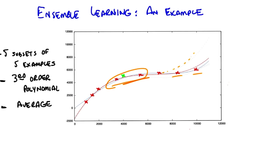
Consider the following algorithm for Bagging (bootstrap aggregation), which is the simplest application of ensemble learning. Bagging involves taking $k$ random samples (with replacement) from the original training dataset, then fitting a model to each sample.

BAGGING ALGORITHM

1. Learn over subset of data.
   • Randomly sample (uniformly + with replacement) subsets of the data.
   • Apply learning algorithm (e.g., decision tree) to each individual subset to yield one fitted model per subset.
2. Combine
   • Continuous Outcome (Regression): mean of model predictions is final output.
   • Discrete Outcome (Classification): mode of model predictions is final output.

Boosting

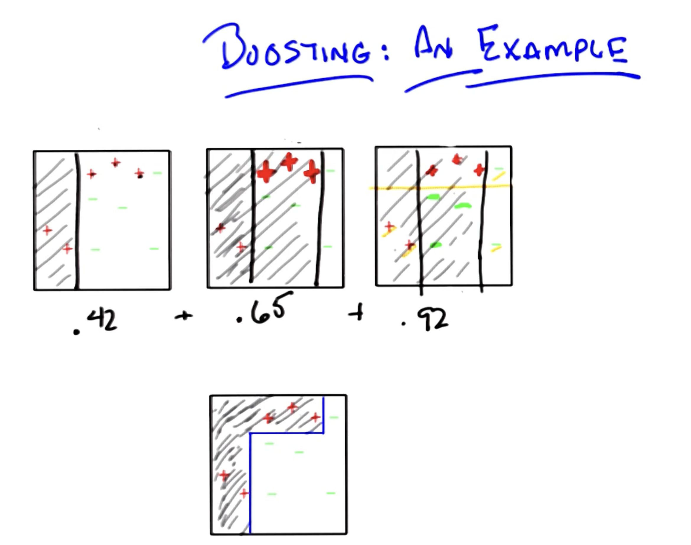
Ensemble Boosting constructs samples in an iterative + sequential fashion, with later samples informed by the results of previous models. This is in contrast to the bagging approach, which constructs samples in a uniformly random fashion.

What do we mean by “informed by the results of previous models”? Given we are on iteration $t$ of boosting, we construct our sampling distribution by upweighting instances that were misclassified in previous iterations. This essentially means we shift the distribution of our sampling towards difficult-to-classify instances.

BOOSTING ALGORITHM

1. Learn over subset of data. LOOP: - Construct new sampling distribution $\mathbb{D}_t$. - Apply learning algorithm to sample $i$ to yield weak learner.
2. Combine $\rightarrow$ weighted combination (weighted mean for regression, weighted majority vote for classification).

Okay, so how does this up-weighting / distribution construction process work?

• For the first iteration, we define a random uniform distribution over training instances.

  \[\mathbb{D}_1(i) = \frac{1}{n}\]

• For all subsequent iterations, we update our previous distribution over instances by shifting up if the instance was misclassified, or shifting down if the instance was classified correctly.

  \[\mathbb{D}_{t+1}(i) = \frac{\mathbb{D}_t(i) \times e^{-\alpha_t y_i h_t(x_i)}}{z_t}\]
  • This formula is defined for binary classification with $y \in \begin{Bmatrix} -1 & +1 \end{Bmatrix}$.
    • In the case of misclassification, $y_ih_t(x_i) = -1$ and $e^{-\alpha_ty_ih_t(x_i)} > 1$. This results in the new $\mathbb{D}_{t+1}(i)$ increasing relative to $\mathbb{D}_t(i)$.
    • In the case of correct classification, $y_ih_t(x_i) = +1$ and $0 < e^{-\alpha_ty_ih_t(x_i)} < 1$. This results in the new $\mathbb{D}_{t+1}(i)$ decreasing relative to $\mathbb{D}_t(i)$.
  • $\alpha_t$ is a function of epsilon defined as part of our weak learner criteria.
  \[\epsilon_t = \Pr_{\mathbb{D}_t}[h_t(x_i) \neq y_i]\] \[\alpha_t = \frac{1}{2} \ln \frac{1 - \epsilon_t}{\epsilon_t} ~~~~~ \alpha_t > 0\]
  • $z_t$ is a normalization constant; all we should know is that $z_t$ depends on the calculation being done at $t$, and is used to ensure the resulting distribution is valid.

Note there are certain special cases. If all instances are misclassified (or similarly, correctly classified), all instances will be upweighted (or down-weighted) to the same degree, resulting in no change from $\mathbb{D}t(i)$ to $\mathbb{D}{t+1}(i)$!

The final hypothesis $H(x)$ is the sign of the weighted sum of the weak learners.

\[H(x) = \text{sign} \left ( \sum_{t=1}^{T}\alpha_t h_t(x) \right )\]

To conclude boosting, consider the following illustrative example. We are dealing with binary classification ($+$ or $-$), and may only use axis-aligned semi-planes to represent decision boundaries (i.e., hypotheses).

---

(all images obtained from Georgia Tech ML course materials)