ML M7: Kernel Methods and SVMs

What are Support Vector Machines?

Definition

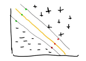
A Support Vector Machine (SVM) is a supervised learning algorithm which calculates the maximally-separating hyperplane to generate predictions. SVMs are best explained in the context of binary classification. Given data $<(x_i, y_i)>$ with $x \in R^{2}$ and $y \in \begin{Bmatrix} -1 & +1 \end{Bmatrix}$, an SVM calculates the hyperplane which maximally separates the two classes. If our data is linearly separable, this might look as follows:

Algorithm

Mathematically, we define the separating hyperplane as a linear combination of input features $x$ and weights $w$. By setting the output to 0, we define the class boundary - any instance yielding a positive output is predicted as the positive class, while instances corresponding to negative output are predicted as the negative class. \(w^Tx + b = 0\)How can we solve for our weight vector? SVMs define a constrained optimization problem, where we are interested in correctly classifying all instances (1) while maximizing the distance between classes, otherwise known as the margin (2).

\[y_i (w^Tx_i + b) \geq 1\tag{1}\] \[\max \frac{2}{||w||} \tag{2}\]

The representation for margin shown above may seem strange, but is directly derived from the difference between support vectors for positive and negative classes. Given the boundary instances of the positive and negative classes $x_1$ and $x_2$…

\[w^Tx_1 + b = 1 ~~~~ w^Tx_2 + b = -1 \tag{1}\] \[\text{Difference}: ~~~ w^T(x_1 - x_2) = 2\tag{2}\] \[\text{Margin}: ~~~ \frac{w^T(x_1 - x_2)}{||w||} = \frac{2}{||w||}\tag{3}\]

Instead of maximizing the margin, we typically reframe our problem to minimize the L2 norm of $w$ - this yields a quadratic programming problem which is more easily solvable.

\[\min \frac{1}{2} ||w||^2\]

With a bunch of hand-waving and blind faith, this enables us to convert our problem to the following maximization over $W(\alpha)$. The key idea here is that this equation is the primary driving force behind SVMs; we will not consider its derivation.

\[\max \left [ W(\alpha) = \sum_i \alpha_i - \frac{1}{2} \sum_{i, j} \alpha_i \alpha_j y_i y_j x_i^Tx_j \right ]\] \[\alpha_i \geq 0 ~~~~ \sum_i \alpha_i y_i = 0\]

From this equation, we know the following:

• We can recover the optimal weight vector $w = \sum_i \alpha_i y_i x_i$
• $\alpha$ is a sparse vector, meaning the majority of data points do not impact our weight vector. This mathematically reflects the notion that only support vectors are required for deriving the weight vector.

Considerations

There are two primary issues with the algorithm as described so far. First, what if our data is separable, but not linearly separable?

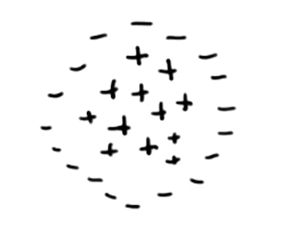
We can use a kernel (window function) to transform our inputs into a higher-dimensional space $\phi(x)$, then apply the SVM algorithm to identify a linear separator in this space. Recall that our optimization equation involves a term to evaluate similarity between points $x_i^Tx_j$. Instead of sequentially applying transformation then SVM algorithm, we can simply swap in a kernel-specific similarity function $K(x_i, x_j)$ to make the process more efficient. This is known as the Kernel Trick.

\[W(\alpha) = \sum_i \alpha_i - \frac{1}{2} \sum_{i, j} \alpha_i \alpha_j y_i y_j K(x_i, x_j)\]

Second, what if no separator exists to completely divide the classes?

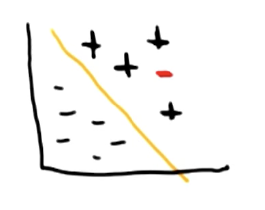
SVMs are typically run as soft-margin classifiers, meaning we allow some misclassification controlled by a slack term $\xi$. The C hyperparameter controls how much misclassification is permissible; smaller values of C result in a softer margin, whereas larger values of C create a harder margin.

\[\min \frac{1}{2} ||w||^2 + C \sum_i \xi_i\]

Back to Boosting

Why don’t we have the issue of overfitting with boosting algorithms?

• As you add more and more weak learners, the algorithm becomes increasingly confident in its predictions. This implies the margin between positive and negative instances becomes increasingly larger.
• Large margins tend to mitigate overfitting!

It is worth noting that boosting will overfit under certain conditions. For example, if each weak learner represents an artificial neural network with many layers and nodes, individual learners will perform too well to realize the benefits of boosting!

---

(all images obtained from Georgia Tech ML course materials)