ML M9: VC Dimension

Issues with Previous Lesson

Review

At the end of the last lesson, we defined Haussler’s Theorem, which provides an upper bound for the number of training instances required to learn a concept in some given hypothesis space $H$.

\[m \geq \frac{1}{\epsilon} \left ( \ln |H| + \ln \frac{1}{\delta} \right )\]

Infinite Hypothesis Space

What happens in the case of an infinite hypothesis space? This occurs more frequently than you might expect - each of the following hypothesis spaces are considered infinite.

• Linear Separators
• Artificial Neural Networks
• Decision Trees w/ Continuous Inputs

Nearly every supervised learning algorithm we’ve discussed so far meets this criterion! Therefore, it would be nice if we had a way to describe the size of a hypothesis space in finite terms.

VC Dimension

Definition

Instead of defining the actual size of a hypothesis space, we can approximate its relative size. For example, Vapnik-Chervonenkis (VC) Dimension defines the power of a hypothesis space as the maximum number of instances it can shatter - label in all possible ways.

Example 1

Consider the following example of VC dimension applied to the infinite hypothesis space of all possible intervals.

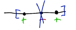
\[\text{Given}: ~~~ H = \begin{Bmatrix} h(x) = x \in \left[a, b \right] \end{Bmatrix}\] \[\text{VC Dimension}: ~~~ 2\]

Given two instances $x_1 = 1$ and $x_2 = 2$, we can define a hypothesis $h(x)$ to label these instances in all possible ways.

\[h_1(x) = [0, 1.5] \rightarrow x_1 = +, x_2 = -\] \[h_2(x) = [1.5, 2.5] \rightarrow x_1 = -, x_2 = +\] \[h_3(x) = [0, 0.5] \rightarrow x_1 = -, x_2 = -\] \[h_4(x) = [0, 3] \rightarrow x_1 = +, x_2 = +\]

Given a third instance, we are not able to generate all possible output label assignments.

Example 2

Next, consider an example more relevant to machine learning. Given a 2-dimensional linear separator, what is the VC dimension?

\[\text{Given}: ~~~ X \in \mathbb{R}^2 ~~~~~ H = \begin{Bmatrix} h(x) = w^Tx \geq \theta \end{Bmatrix}\] \[\text{VC Dimension}: ~~~ 3\]

In this case, we are able to shatter three points in 2D space.

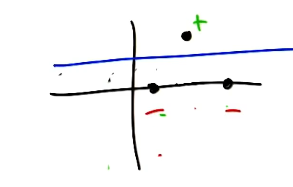
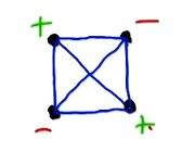
No matter how we arrange four points in this space, there is no way to classify them using every possible combination of outputs.

Conclusions + Application

VC dimension is often equivalent to the number of parameters in the learning algorithm. In the case of an interval, we have two parameters $a$ and $b$. For our 2D linear separator, we have three parameters $w_1$, $w_2$, and $b$. This implies that any d-dimensional hyperplane has $VC = d + 1$.

VC dimension can be applied to sample complexity to yield a more manageable version of Haussler’s Theorem.

\[m \geq \frac{1}{\epsilon} \left ( 8 \times VC(H) \times \log_2\frac{13}{\epsilon} + 4\log_2\frac{2}{\delta} \right)\]

Furthermore, we can define the upper bound of VC dimension for a finite hypothesis space.

\[d \leq \log_2|H|\]

Finally, H is PAC-learnable if and only if VC dimension is finite.

---

(all images obtained from Georgia Tech ML course materials)