NLP M12: Machine Translation

Machine Translation Basics

Machine Translation is the process of translating a document from one language into another.

A Brief History of Machine Translation

Machine translation and artificial intelligence have a lengthy history, with particular reference to the contributions of Alan Turing involving World War II code breaking during the mid 1940s. By 1954, IBM had produced a functional translation of a 60-second audio clip spoken in Russian to English. Still, roadblocks were encountered, leading to the 1960 suggestion that high-quality machine translation requires a more effective understanding of meaning. Ultimately, the ALPAC Report in 1966 declared human translation as cheaper and better than machine translation, shutting down most efforts for the next few decades.

In 1990, IBM produced the first statistical machine translation system known as IBM CANDIDE. Further progress was made in statistical and phrase-based machine translation over the 2000s, eventually leading to the development of neural machine translation in the 2010s.

Problems

Machine translation is a particular difficult task for a number of reasons:

• Words are not guaranteed to have a one-to-one correspondence, and may be re-ordered.
• Phrases in one language may be split into multiple phrases in other languages.
• Words have different meanings in different contexts.
• The degree of lexical specificity can differ across languages.
• Different languages have different structures (ex: Subject-Verb-Object vs. Subject-Object-Verb).
• Negation mechanics differ by language.

General Approach

In a perfect world, we would have some perfect intermediate language that could express all thoughts and knowledge. Then, translation would involve mapping from source to intermediate, followed by intermediate to target. Unfortunately, all languages have some level of imprecision - particularly through semantic ambiguity - which prevents us from taking this approach.

So how can we get from a source to target language? We can still get to some intermediate form via analysis, then get to our target via generation. More formally, this process is represented by the Vauquois Triangle. Although we cannot reach the perfect interlingua, we can select some level of analysis to serve as a “shortcut” for jumping from source to target.

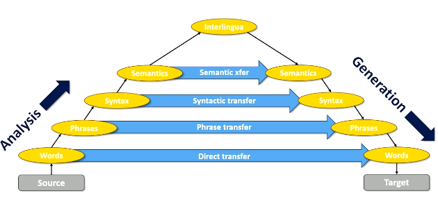
• Direct Transfer: word-to-word translation. Probabilistic mapping.
• Phrase Transfer: map phrases in one language to phrases in another. Probabilistic mapping.
• Syntactic Transfer: estimate probability of syntax tree for target given syntax tree in source.

Recall we can formulate our translation problem in terms of Bayes Rule:

\[\Pr(s_t ~ | ~ s_s) \propto \Pr(s_s ~ | ~ s_t) \times \Pr(s_t)\]

• Language to Language Probability: $\Pr(s_s ~ | ~ s_t) \rightarrow$ is our translation faithful / accurate?
• Fluency in Target Language: $\Pr(s_t) \rightarrow$ is our translation fluent? Recall this term can be broken down into a Markov Chain as $\Pr(s_t) = \Pr(w_1, \ldots, w_n) = \prod_n \Pr(w_n ~ | ~ w_{n-1})$.

We’ve spent considerable time modeling the fluency of a body of text, but how can we estimate language-to-language probability? This task requires a collection of parallel corpora - a body of text with the same meaning but written in different languages. The most famous example of a parallel corpora is the Rosetta Stone!

Machine Learning Considerations

Evaluation

Before discussing specific model implementations, let’s establish a baseline for evaluating translations. Machine translation evaluation involves balancing two components:

• Fidelity: does the translation capture all information in the source?
• Acceptability: does the translation capture enough of the source to be useful?

So how can we calculate terms for these values? In a non-automated setting, we can use human evaluation to subjectively rank translations. However, this is quite expensive and not ideal for automation.

Instead, Bilingual Evaluation Understudy (BLEU) Score is commonly applied to translations to compute a quantitative score. BLEU score is the geometric mean of 1- to n-gram precision multiplied by a brevity penalty. More specifically…

• Given predicted and reference translations, we compute the ratio of n-gram appearances in predicted versus reference. This is repeated for all possible n-grams.
• The geometric mean is taken across n-grams.

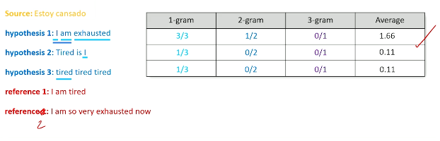
The complete BLEU score is calculated as geometric mean $\times$ brevity score.

\[BLEU = BP \times \exp(\sum_{n=1}^N \frac{1}{n} \log p_n)\]

• $p_n$: proportion of n-grams present in references.
• $n$: specific n-gram currently being considered; we typically use $N=4$.
• $BP$: brevity penalty; calculate using $r =$ length of reference and $c =$ length of prediction.

\[BP = \begin{cases} 1 & c > r \\ e^{(1 - \frac{r}{c})} & c \leq r\end{cases}\]

Machine Translation as Transfer

Recall that we can define machine translation based on analysis level:

• Direct Transfer: word-to-word granularity of translation.
• Phrase Transfer: phrase-to-phrase granularity of translation.

Transfer tends to work better when working with chunks of text, since word-to-word translation is often problematic in terms of ordering / context. However, this is not always the case, but rather highly dependent on the context + word(s) in consideration.

What sort of problems do we need to account for in our modeling system?

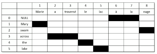
• Word Alignment: every source word $s_i$ is aligned to one target word (including NULL) $t_j$ such that $a_i = j$.
  • we bundle in word alignment to our probabilistic representation of translation quality.

\[\Pr(t ~ | ~ s) = \sum_a \Pr(t, a ~ | ~ s) = \sum_a \Pr(t ~ | ~ a, s) \times \Pr(a)\]

• Phrase Transfer vs. Word Transfer: when should we choose to translate phrases vs. words?
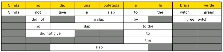
  • We can construct a phrase lattice to represent all possible combinations of phrase vs. direct word translations. Note that the phrase lattice contains the results of direct transfer as the first row, then possible alternative phrase translations in subsequent rows.
  • Once we have the full phrase lattice, our computation becomes an argmax over the probability of observing each possible sequence of translation terms.

\[\arg \max_t \prod_{(s, t)} \Pr(s ~ | ~ t) \times \prod_{i=1}^t \Pr(t_i ~ | ~ t_{i-1}, \ldots)\]

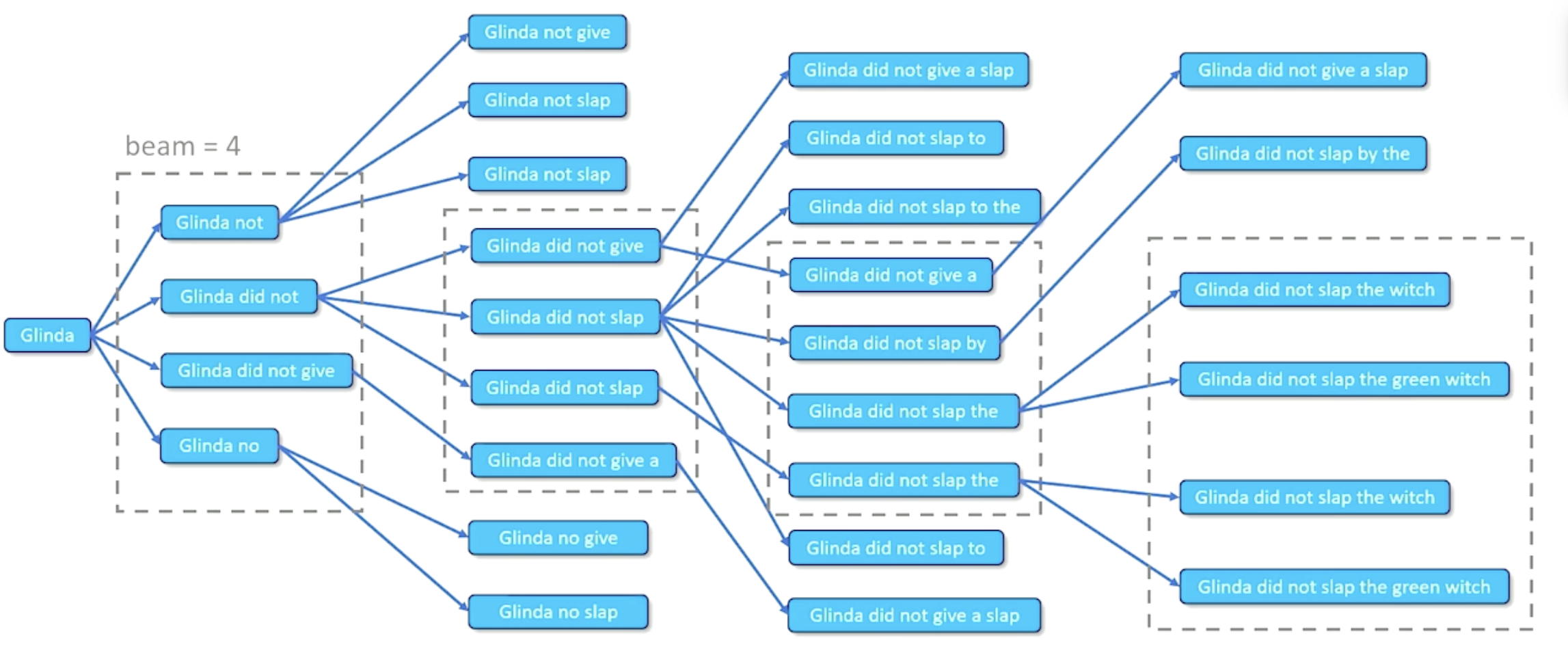
What happens when we have massive phrase lattice tables, and computational demand becomes infeasible? Beam Search reduces our search space by maintaining a fixed number of paths $k$ - more specifically, the top $k$ scoring options - at each step forward in sequence generation.

Neural Machine Translation

Current state-of-the-art approaches for machine translation involve Neural Networks - shouldn’t be a huge surprise at this point! Recall that Recurrent Neural Networks (RNNs) process a sequence of items, generating some hidden state at each time step used in the prediction for the next time step. Long Short-Term Memory (LSTM) networks have a more complicated hidden state representation, which tends to transfer to better results.

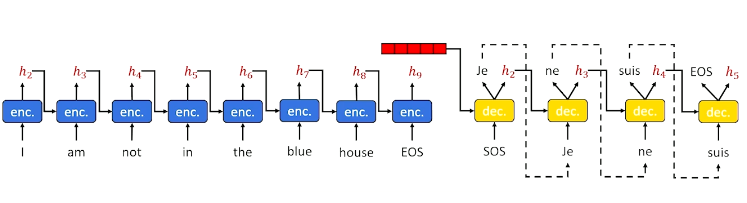
Unfortunately, vanilla RNNs / LSTMs generate terms in a sequential (left-to-right fashion). This is not always appropriate in the case of translation, where we may need to perform word re-ordering / re-selection depending on future terms in the source language. Instead, Sequence-to-Sequence (seq2seq) networks are more appropriate for this application. Recall that seq2seq networks follow an encoder-decoder neural architecture, where the encoder iteratively processes every term in the source to generate some final informative hidden state. This implies the hidden state passed to the decoder for generation will have access to all semantic information in the source sequence.

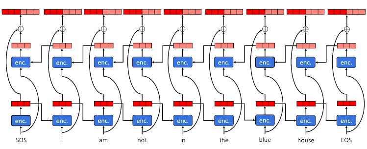
Still, basic seq2seq networks encode in a sequential left-to-right fashion. Since translation involves reordering, we may want to also have right-to-left context in order to have a more comprehensive representation of semantic meaning. Bidirectional seq2seq models generate two sets of hidden states as part of the encoder: a set from left-to-right, and a set from right-to-left. The final hidden state for each time step is the concatenation of the corresponding left-to-right and right-to-left hidden states.

Bidirectional seq2seq with attention was considered state-of-the-art until the emergence of today’s cutting edge: the Transformer. Recall that transformer architecture involves the following key components:

• Encoder-Decoder structure.
• Self and Multi-Headed Attention.
• Random masking to generate meaningful word embeddings.

In practice, transformers for machine translation are often trained as multi-lingual using many parallel corpora. Generated pre-trained transformers (e.g., GPT) tend to perform reasonably well at translation, but transformers explicitly trained for the target task of translation are often better.

---

(all images obtained from Georgia Tech NLP course materials)