NLP M5: Semantics

Document Semantics

Semantics refers to the meaning of words and phrases. This is particularly straightforward to humans, but difficult for computers to represent. For example, does a dictionary “know” what a given word means, even if it contains the precise definition of the word?

We are often interested in understanding the semantics of a document, which is a collection of words. Recall that we can represent any word as a one-hot vector; we can extend this representation to documents using a multi-hot vector, which assigns 1 for every word appearing in the document. This is a good starting point, but isn’t very effective at capturing document semantics.

Document Similarity

Given two or more documents, how can we determine if the content of the documents is similar? First, we need a good metric for measuring document semantics.

TF-IDF

Term Frequency-Inverse Document Frequency (TF-IDF) is an approach which assigns relative weight to each word based on its importance within the document. TF-IDF has two core components:

• Term Frequency: frequency of a word within a document; if a word shows up more frequently in a document, it should be more important.
  $TF(w, d) = \log(1 + freq(w, d))$
• Inverse Document Frequency: inverse of word frequency across all documents in consideration; words that are common across all documents should not have high importance. $IDF(w, d) = \log\frac{1 + |D|}{1 + freq(D, w)} + 1$
  • $D$ : number of documents in “all documents” set.
  • $freq(d, w)$ : number of documents in which word $w$ appears.

Note that both the $TF$ and $IDF$ terms contain +1 constants for smoothing, which ensures that a frequency of 0 does not break the equation. Finally, TF-IDF is a combination of these two components:

\[\text{TF-IDF}(w, d, D) = \text{TF}(w, d) \times \text{IDF}(w, D)\]

We can apply TF-IDF to each word in our vocabulary, for each document in our set. This yields a vector of TF-IDF scores per document.

Document Retrieval

Once we have a vector representation of our documents, we can move to assessing document similarity. Document similarity has many practical applications - for example, Document Retrieval is the process of using a word or phrase (considered a document) to query another set of documents and return the most similar results.

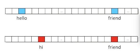
How do we calculate similarity? First, let’s assume we are using a multi-hot representation of documents. Consider the following two documents: “hello friend” and “hi friend”.

We can plot these vectors in Cartesian Space and use Euclidean Distance to calculate their straight-line distance.

\[||a - b|| = \sqrt{\Sigma_i(a_i - b_i)^2}\]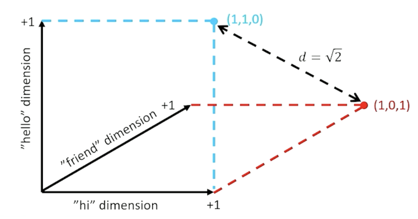

Other distance metrics such as Cosine Similarity tend to be more popular in practice.

\[\cos(a, b) = \frac{a \cdot b}{||a|| * ||b||}\]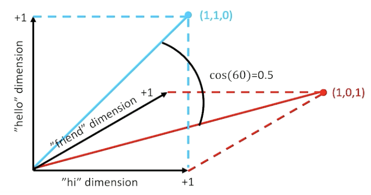

With this context in mind, document retrieval proceeds as follows:

1. Create a $1 \times |V|$ normalized document vector for the query $q$.
2. Create a normalized vector for every document in the set, and stack to create a $D \times V$ matrix $M$.
3. Matrix multiply $q \cdot M$ to calculate similarity scores; this is the same as computing cosine similarity.
4. Identify the documents with top $k$ scores.

Word Embeddings

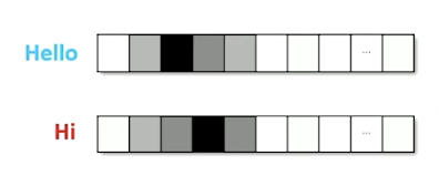
Multi-hot and TF-IDF document representations still struggle to capture simple semantics. For example, both strategies fail to recognize that “hi” and “hello” have the same meaning. Is there another strategy we can use here?

Embedding Representation

Word Embeddings use a linear transformation to find a more compact representation of the original input word. Instead of using a $|V|$-dimensional space, we create a transformed $d$-dimensional space that intuitively maps similar words and phrases close together.

The concept of embedding can be applied within broader neural architectures; for example, encoders within RNNs commonly use embeddings as the first layer.

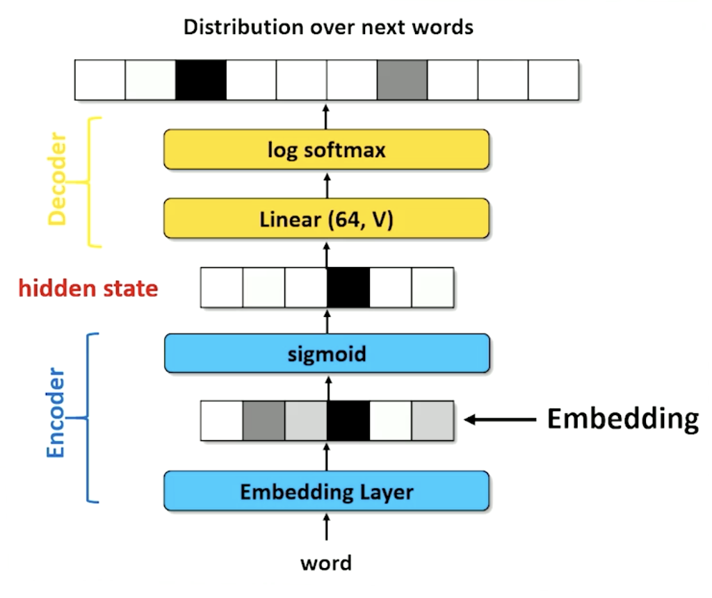
An embedding layer is essentially a linear layer nn.Linear(|V|, d), but note that our linear transformation is different than usual. Since we are guaranteed a $|V|$-dimensional one-hot vector as input, our linear transformation essentially “looks up” the weights corresponding the the one-hot index for the word within the $|V| \times d$ weight matrix. For this reason, deep learning libraries implement more efficient modules for this task, such as nn.Embedding(|V|, d) within torch.

Word2Vec and Distributional Semantics

As currently presented, embeddings are task-specific. The transformation is learned within the context of some broader neural network, which operates on the target task of interest. Can we generalize the embedding process to find a general method for converting a word to a vector, and make it task-agnostic?

We can use Distributional Semantics to define embeddings centered on surrounding words. Distributional semantics refers to the idea that we don’t actually need to know the dictionary definition of a word to represent its semantic meaning. Instead, “a word is known by the company it keeps” - words that are surrounded by similar words tend to have similar meaning.

Word2vec is a neural network approach to creating word embeddings through the use of distributional semantics. Word2vec frames embedding as one of two classification problems:

• Continuous Bag of Words: predict a single masked word in the context of surrounding words. “You will find the crown with the __ when in the throne room.”
• Skip-Gram: predict many surrounding words from a single word. “__ __ __ queen __ __ __.”

As a result of the embedding process, words that represent similar concepts should be clustered closely in the $d$-dimensional embedding space.

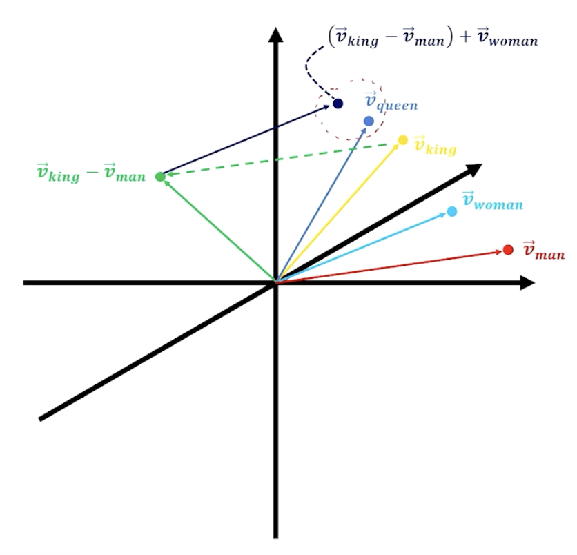
Document embeddings are the sum over all word embeddings for words within the document.

---

(all images obtained from Georgia Tech NLP course materials)