RL M1: Intro to Reinforcement Learning
Module 1 of CS 7642 - Reinforcement Learning @ Georgia Tech.
Walkthrough of RL Components (Smoov and Curly)
Example RL Problem: Grid World
Recall from CS 7641: Machine Learning that the simplest example of an RL problem is Grid World, which defines a grid-based world which an agent must navigate through to get to a goal state.
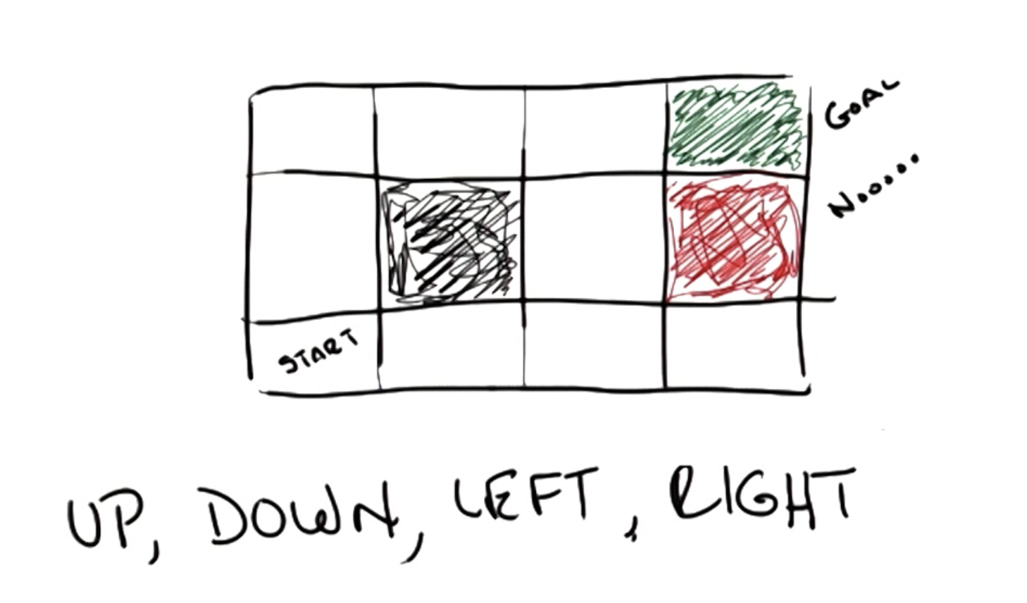
We introduce stochasticity into our world such that actions do not always result in the desired consequences.
\[\Pr(a) = \begin{cases} a ~\text{executes as desired} & 0.8 \\ \text{action} ~ 90^o ~ \text{to left executes} & 0.1 \\ \text{action} ~ 90^o ~\text{to right executes} & 0.1 \end{cases}\]Markov Decision Process
The Markov Decision Process (MDP) is a formal mathematical representation for a reinforcement learning problem. MDPs involve a decision-making agent interacting with its environment. Any MDP is defined by the following components:
- States $s \in S$: set of possible states in which the environment exists.
- Actions $a \in A(s)$: set of possible actions available to agent for a particular state.
- Model $T(s, a, s’) \sim \Pr(s’ | s, a)$: defines the probability of transitioning from state $s$ to state $s’$ as a result of some particular action $a$.
- The model captures any stochasticity to our world, and is our attempt to directly model the underlying “physics” of world behavior.
- Reward $R(s), R(s, a), R(s, a, s’)$: function mapping environmental state $s$ (in conjunction with other components, if necessary) to numerical reward.
The solution to an MDP is a Policy, which is a mapping from every possible state to an action. A policy is basically a reference guide for an agent to follow when navigating through the RL problem, indicating which action to take when presented with a particular environmental state.
\[\pi(s) \rightarrow a\]There are two key assumptions to MDPs:
- As part of the Markov Property, we assume the current state is only depending on previous state (as opposed to the sequence of previous states). In other words, the future is independent of the past given the present.
- Specific statistical components of the MDP (e.g., model / transition function) are stationary, meaning their properties do not change over time.
Rewards
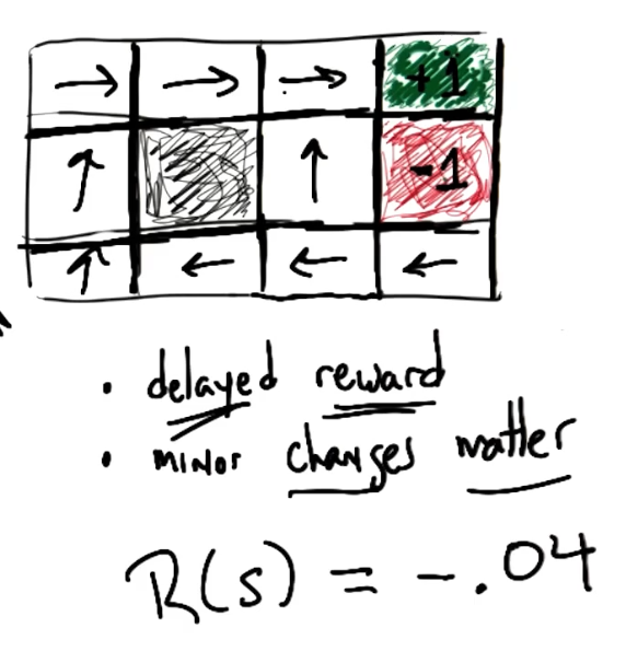
In the context of MDPs, a Reward is a numerical signal from the environment indicating the level of consequence (good or bad) for an action. The agent receives reward from the environment at each time step of the MDP. This framework gives rise to the temporal credit assignment problem, which refers to the difficulty of attributing reward to a particular action given that 1) reward is often delayed, and 2) any episode of an MDP involves selecting a series of actions.
Minor changes to reward structure have massive impacts on the optimal solution! Therefore, domain knowledge / subject matter expertise is often bundled into reward definition by the MDP creator in order to produce desired behavior. For example, if we would like to encourage our Grid World agent to reach the goal state as soon as possible, we might assign small negative reward to each intermediate state.
Assumptions
We’ve been making two key assumptions as part of our overview of MDPs:
Infinite Horizons: the agent has an infinite number of time steps to interact with the environment. The reverse case - finite horizons - is often more suitable in practice. Without the notion of infinite horizons, we may lose stationarity with regards to our policy.
\[\text{Infinite Horizons} ~~ \pi(s) \rightarrow a\] \[\text{Finite Horizons} ~~ \pi(s, t) \rightarrow a\]Utility of Sequences: given two action sequences both beginning in the same state $S_0$ but immediately diverging thereafter, with sequence $1$ having greater total utility (value) than sequence $2$, we assume that the sequence of states following $S_0$ for sequence $1$ is better than that for sequence $2$.
- This seems obvious, but does raise question to our definition of “utility”.
Utility = Value
Utility - better known as Value in most RL material - is the combined reward corresponding to a sequence of states and/or actions. Put more simply, is considered the total expected reward beginning in a certain state.
Our simplest definition of utility is the sum of rewards across states.
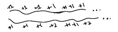
\[U(S_0, S_1, \ldots) = \sum_t R(S_t)\]However, this definition fails in the case of infinite horizons. For example, how do we compare the value of two infinite sequences with only positive reward? In both cases, we have $U = +\infty$.
To fix this situation, we calculate utility as cumulative discounted reward. This enables us to place an upper bound on utility, thereby assigning finite value to an infinite series!
\[U(S_0, S_1, \ldots) = \sum_t \gamma^{t} R(S_t) \leq \frac{R_{\text{MAX}}}{1-\gamma}\]The key distinction between reward and utility is immediate vs. long-term gratification. Reward is a single value associated with a particular state; utility is the expected cumulative discounted reward starting from a particular state.
Policies
Recall that we’ve defined a policy as some comprehensive mapping from states to actions. In other words, a policy assigns action to each possible state in our MDP $s \in S$.
\[\pi(s) \rightarrow a ~~ \forall s \in S\]How do we solve for the optimal policy? Given our definition of value, we can now define the optimal policy in terms of expected discounted cumulative reward.
\[\pi^{*} = \arg \max_{\pi} \mathbb{E} \left[ \sum_t \gamma^{t} R(S_t) | \pi \right]\] \[\pi^{*}(s) = \arg \max_a \sum_{s'} T(s, a, s') V_{\pi^{*}}(s')\]We define the utility (value) $V(s)$ of entering a particular state as the expected discounted cumulative reward proceeding from this state (1). Given our formula for the optimal policy, we can substitute / rearrange to yield a more usable representation known as the Bellman Equation (2)!
\[V_{\pi}(s) = \mathbb{E} \left [ \sum_t \gamma^{t} R(S_t) | \pi, S_0 = s \right] \tag{1}\] \[V(s) = R(s) + \gamma \max_a \sum{s'} T(s, a, s') V(s') \tag{2}\]How do we solve the Bellman Equation? We have a system of equations…
- $n$ equations $\rightarrow$ value $V(s)$ for each state in our state space $s \in S$, with $|S| = n$.
- $n$ unknowns $\rightarrow$ each value $V(s)$ is an unknown variable.
Unfortunately, we cannot solve using a system of linear equations due to the non-linear $\max$ component in each equation. How can we solve our problem, then?
Solving MDPs
Value Iteration
Value Iteration involves iteratively approximating the state-value function until converging to stable estimates.
\[\hat{V}_{t+1}(s) = R(s) + \gamma \max_a \sum_{s'} T(s, a, s') \hat{V}_t(s')\]Initialize state utilities $V(s)$ to random values. Loop until convergence:
- For each state $s \in S$, update utility estimate based on current set of utility estimates.
Once we have our final estimates for state value, we can recover the optimal policy by simply walking through our state space!
Policy Iteration
Instead of estimating the value function (to then derive the optimal policy), we can directly estimate the policy through methods such as Policy Iteration.
\[V_t(s) = R(s) + \gamma \sum_{s'} T(s, \pi_t(s), s') V_t(s') \tag{1}\] \[\pi_{t+1} = \arg \max_a \sum_{s'} T(s, a, s') V_t(s') \tag{2}\]Initialize state utilities $V(s)$ to random values. Initialize policy $\pi_0$ to random guess. Loop until convergence:
- Evaluate: given $\pi_t$ calculate $V_t(s)$ by following this policy (Equation 1 below).
- Improve: define updated policy $\pi_{t+1}$ by stepping through state space (Equation 2 below).
Policy iteration directly addresses the non-linearity present in the original Bellman Equation. This means we can perform the evaluation step by solving a system of linear equations!
More on the Bellman Equation
The most traditional version of the Bellman Equation is defined in terms of state value.
\[V(s) = \max_a \left[R(s, a) + \gamma \sum_{s'} T(s, a, s') V(s')\right]\]Another version focuses on state-action value.
\[Q(s, a) = R(s, a) + \gamma \sum_{s'} T(s, a, s') \max_{a'} Q(s', a')\]Why bother to define a second equation? It turns out the $Q$ form is very useful in the context of reinforcement learning - this is because $Q$ enables us to take expectations using only experienced data, whereas $V$ requires well-defined structures for $R(s, a)$ and $T(s, a, s’)$. This distinction is the basis of model-free vs. model-based methods in reinforcement learning, respectively.
(all images obtained from Georgia Tech RL course materials)