RL M2: RL Basics
Module 2 of CS 7642 - Reinforcement Learning @ Georgia Tech.
Problem Setup
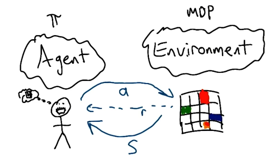
Most problems in reinforcement learning (RL) are presented in terms of two key entities:
- Agent: the decision-making, action-taking entity within our model world.
- Environment: everything outside the agent’s control which impacts state transitions and rewards.
The agent selects actions $a$ to take within the environment. As a result, the environment provides the agent with an updated state $s \in S$, as well as some indication of action evaluation represented as numeric reward $R(s, a) \in \mathbb{R}$.
Mystery Game
Consider the following game for the purposes of RL demonstration. We define a grid-based game in which the agent is not aware of the specific rules. The agent selects actions $a \in \begin{Bmatrix} 1 & 2 & 3 & 4 & 5 & 6 \end{Bmatrix}$.
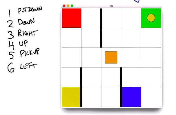
How could our agent discover the rules of the game? It would be most appropriate to start taking random actions, then progressively figure out what works (higher reward) versus what doesn’t. It turns out this game is very well-known - it’s the classic Taxi Cab game used as a toy example in RL!
RL Algorithms
Behavior Structures
As part of agent-environment interaction, our agent should learn some Behavior which is desirable in the context of reward. There are different types of behavior
- Plan: fixed sequence of actions; open-loop sequence that does not account for state feedback.
- Conditional Plan: sequence of actions which depends on the environment. For example, $\text{if (this)} \rightarrow^{\text{then}} \text{do that}$
- Stationary Policy: comprehensive mapping from states to actions. Handles stochasticity of environment very well, since the policy is a function of environmental state $\pi(s) \rightarrow a$.
- Useful for defining full range of behavior, but may be unnecessary for vast state spaces where agent is not likely to end up in certain states.
Our learning algorithms should return an optimal policy. But how do we define optimal?
Evaluating a Policy
We can evaluate a policy by evaluating the sequence of states which it selects as part of a trial. This might work as follows:
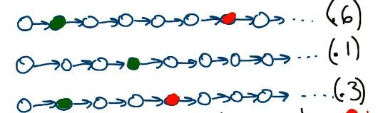
- Define immediate rewards for each transition $R(s)$.
- Truncate according to horizon (in the case of finite horizon).
- Summarize sequence with single number (sequence return $= \sum_i \gamma^{i}r_{t+i+1}$).
- Summarize over sequences (average sequence return).
Look familiar? This is the same general idea as presented in the previous lesson, but framed in a slightly different way. The average sequence return is better known as expected cumulative discounted reward in the context of RL.
Evaluating a Learner
Given that a policy is the output of a learning algorithm, how can we evaluate the quality of the learning algorithm itself? We could define quality from a number of perspectives:
- Value of returned policy
- Computational complexity (execution time)
- Sample complexity (amount of data = experience required to learn)
Although we typically discuss space complexity in the context of algorithms, it is not particularly interesting in the context of RL since it is typically not a limiting factor.
(all images obtained from Georgia Tech RL course materials)