RL M3: TD and Friends
Module 3 of CS 7642 - Reinforcement Learning @ Georgia Tech.
RL Context
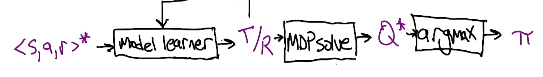
Experience in reinforcement learning (RL) typically comes in the form of state-action-reward tuples. We feed this data into an RL algorithm to find the optimal policy. \((s, a, r)_i \rightarrow ~ \text{RL Algorithm} ~ \rightarrow \pi\) There are three main families of RL algorithms:
- Model-Based: use input experience to learn some representation of the model (state transition and reward functions), which is then used to solve a Markov Decision Process (MDP).
- Model is iteratively learned from experience.
- Once model is learned, we can directly solve for the optimal value function, which is then used to derive the optimal policy.
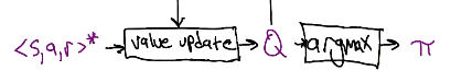
- Model-Free: use input experience to iteratively learn the value function, which is then used to derive the optimal policy.
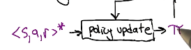
- Policy Search: instead of using any model or value function component, we directly estimate the policy in an iterative fashion.
- The learning problem is very difficult, since the feedback we get regarding our current estimate of the policy may not be sufficient.
Different problems have different characteristics, meaning the “best” algorithm is highly dependent on the problem. Most RL research focuses on model-free approaches since it strikes a nice balance between computational simplicity and effective learning updates.
TD Learning
Prediction vs. Control
In the context of reinforcement learning, prediction refers to the task of estimating the value function. This is in contrast to control, where the objective is to define some policy to control an agent’s actions.
Temporal Differences
Temporal Difference (TD) Learning is a model-free prediction method which incrementally learns the value function using estimates from sequential estimates. TD Learning is considered a bootstrapping method since it updates estimates based on other learned estimates.
Recall that an RL problem involves collecting experience in the form of $(s, a, r)_i$ instances. Instances collected within an episode - or single trial of an MDP - correspond to time steps.
\[s_0 \rightarrow^{a_0} r_0~~ s_1 \rightarrow^{a_1} r_1 ~~ s_2 ~~ \ldots ~~s_{k-1} \rightarrow^{a_k} r_k ~~ s_F\]In addition to time steps within an episode, we also have the episodes themselves. This means we can define two types of sequences - one corresponding to estimates within time steps of an episode, and the other corresponding to estimates across entire episodes. In the following section, we will consider how TD Learning can perform incremental learning using sequences of 1) entire episodes, 2) time steps within an episode, and 3) a combination of the two!
TD(1) - Incremental Learning across Episodes
How do we estimate the value of a state across episodes? Value is defined as the expected discounted cumulative reward for a state. To calculate using episodic data, we might simply take the average of discounted cumulative reward for each state observed across episodes.
\[\text{Let} ~ R_t(s) = ~ \text{actual discounted cumulative reward for episode} ~ T\] \[V_T(s) = \frac{1}{T} \sum_T V_t(s)\]To learn value in an incremental fashion, we simply re-take the average of the value function with each additional episode $(1)$. We can reorganize this equation to yield an update process similar to the perceptron rule $(2)$.
\[V_T(s) = \frac{(T-1) V_{T-1}(s) + R_T(s)}{T} \tag{1}\] \[V_T(s) = V_{T-1}(s) + \alpha_T \left( R_T(s) - V_{T-1}(s) \right) ~~~~~~ \alpha_T = \frac{1}{T} \tag{2}\]Note that $R_T(s) - V_{T-1}(s)$ represents the error between the actual discounted cumulative reward observed at episode $T$ and the previous estimate of the value function at episode $T-1$.
The full equation shown in $(2)$ is the TD(1) Update Rule, which performs updates by averaging across episodes. See below for the TD(1) algorithm - although this form looks a bit different, it calculates the same value as above.
Episode T
For all $s, e(s) = 0$ at start of episode, $V_T(s) = V_{T-1}(s)$
After $s+1 \rightarrow^{r_t} s_t$: (time step $t$)
$e(s_{t-1}) = e(s_{t-1}) + 1$
For all $s$:
$V_T(s) = V_T(s) + \alpha_T(r_t + \gamma V_{T-1}(s_t) - V_{T-1}(s_{t-1}))e(s)$
$e(s) = \gamma e(s)$
TD(1) involves incremental learning across episodes, which may be problematic depending on our data. For example, what if we only observe certain states a few times across all episodes? Our experienced trajectories may bias the results to a problematic degree. For example, if we start in state $s_2$ a single time, but experience great discounted cumulative reward due to getting “lucky”, our estimate of $s_2$ will be much higher than that for a model-based approach.
\[V(s_2) = 2 + \gamma \times 0 + \gamma^2 \times 10\]
TD(0) - Incremental Learning across Time Steps
TD(0) Learning performs incremental updates across time steps within an episode, which corresponds to the maximum likelihood estimate of value for a particular state.
\[V_T(s_{t-1}) = V_T(s_{t-1}) + \alpha_T(r_t + \gamma V_T(s_t) - V_T(s_{t-1}))\]In contrast to TD(1), TD(0) uses intermediate estimates obtained for neighbor states to update the value of a current state within an episode. This means we do not wait until the end of an episode to perform updates, but are rather informed by each time step within an episode.
\[\text{TD(0)}: ~~ V_T(s_{t-1}) = \mathbb{E} \left[r_t + \gamma V_T(s_t) \right]\] \[\text{TD(1)}: ~~ V_T(s_{t-1}) = \mathbb{E} \left[r_t + \gamma r_{t+1} + \gamma^2 r_{t+2} + \ldots \right]\]The TD(0) algorithm is summarized below.
Episode T
For all $s, V_T(s) = V_{T-1}(s)$
After $s_{t-1} \rightarrow^{r_t} s_t$: (step $t$)
For all $s$:
$V_T(s) = V_T(s) + \alpha_T(r_t + \gamma V_{T-1}(s_t) - V_{T-1}(s_{t-1}))$
TD($\lambda$) - Combination of TD(0) and TD(1)
Both TD(0) and TD(1) have updates based on differences between temporally successive predictions. We can define a more general approach known as TD($\lambda$), where TD(0) and TD(1) are considered special cases.
TD($\lambda$) blends updates to the value function on a spectrum between 1) purely time-step-based and 2) purely episode-based. The $\lambda$ hyperparameter controls the influence of the eligibility trace on state updates across time steps.
- In the case of TD(0) $\rightarrow$ $e(s) = 1 ~ \forall s \in S$
- In the case of TD(1) $\rightarrow$ $e(s)$ decays with $\gamma$
- Although difficult to see without derivation, this mathematically results in a purely episodic update rule equivalent to Monte Carlo Learning.
Episode T
For all $s$, $e(s) = 0$ at start of episode, $V_T(s) = V_{T-1}(s)$
After $s_{t-1} \rightarrow^{r_t} s_t$: (step $t$)
$e(s_{t-1}) = e(s_{t-1}) + 1$
For all $s$:
$V_T(s) = V_T(s) + \alpha_T(r_t + \gamma V_{T-1}(s_t) - V_{T-1}(s_{t-1}))e(s)$
$e(s) = \lambda \gamma e(s)$
By tuning $\lambda$, we decide how much we trust our current bootstrapped estimate versus the actual trajectory when estimating the value function.
K-Step Estimators
TD(0) represents the extreme case of updating the value function at each time step. It uses the reward experienced during the time step (as a result of the state transition) in combination with the current estimate of the value of the subsequent state.
\[\text{TD(0)} = E_1: ~~~V(s_t) = V(s_t) + \alpha_T(r_t + \gamma V(s_{t+1}) - V(s_t))\]Conversely, TD(1) represents the extreme case of updating the value function after each episode. It uses the full sequence of observed rewards across the episode to estimate the value of a given state.
\[\text{TD(1)} = E_\infty: ~~ V(s_t) = V(s_t) + \alpha_T(r_t + \ldots + \gamma^{k-1}r_{t+k-1} - V(s_t))\]More generally, any K-Step Estimator uses $k$ time steps of observed rewards to estimate the value function. Any remaining time steps in the episode are bundled into the current value function estimate, therefore relying on bootstrapping.
\[E_k: ~~ V(s_t) = V(s_t) + \alpha_T (r_t + \ldots + \gamma^{k-1} r_{t+k-1} + \gamma^k V(s_{t + k}) - V(s_t))\]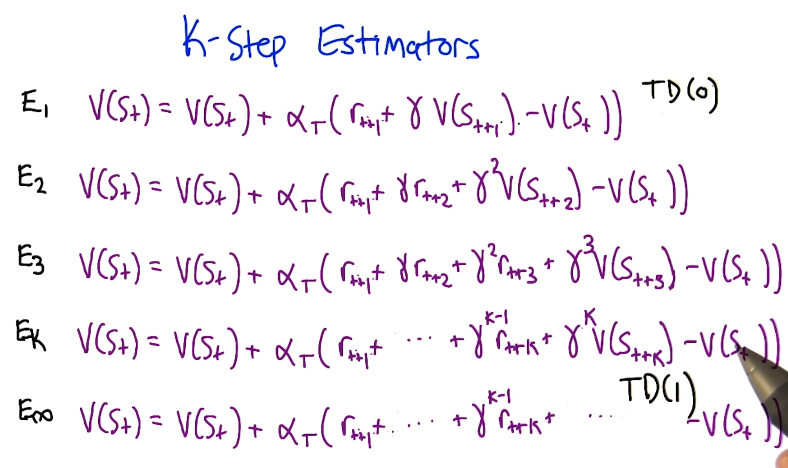
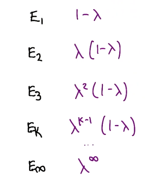
TD($\lambda$) is a weighted combination of all k-step estimators. More specifically, each k-step estimator’s weight is a function of both $k$ and $\lambda$. In the most extreme cases, we get complete weight on either $E_1$ in the case of TD(0) or $E_\infty$ in the case of TD(1).
The best values for $\lambda$ typically fall between $0.3$ and $0.7$. As with any other machine learning algorithm, we should treat $\lambda$ as a tunable hyperparameter which should be optimized relative to the specific problem at hand.
(all images obtained from Georgia Tech RL course materials)