CNN Backprop + Common Architectures

Introduction#

In the previous lesson, we introduced the concept of a Convolutional Neural Network (CNN) and discussed its most common layer types - convolutional and pooling layers - in terms of their forward pass characteristics. The purpose of this lesson is to 1) explore the derivation of a gradient + backwards pass for a convolutional layer, and 2) discuss some basic CNN architectures.

Backwards Pass#

Recall that Backpropagation is the recursive application of the chain rule to the layers of a neural network, with the primary goal of the backwards pass being to calculate the gradient of the loss function w.r.t. the weights of each layer.

Gradient Descent + CNNs#

In order to perform Gradient Descent as part of backpropagation, we need to calculate the gradient of the loss function w.r.t. the weights we wish to update. Put more formally…

$\text{UPDATE STEP}: ~~~ w^{(t+1)} = w^{(t)} + \alpha \times \nabla L(w)$

$\text{GRADIENT CALCULATION}: ~~~ \nabla L(w) = \frac{\partial{L}}{\partial{w}} = \frac{\partial{L}}{\partial{h}} \times \ldots \times \frac{\partial{h}}{\partial{w}}$

As part of CNNs, we have introduced two new layer types: the convolutional and pooling layers. Pooling layers do not have any learned parameters; this implies we do not need to estimate the gradient w.r.t. any weights in a pooling layer. In contrast, convolutional layers contain learned parameters within the kernel. We will need to calculate the gradient of the loss function w.r.t. weights of the kernel, which can be represented as $\frac{\partial{L}}{\partial{k}}$.

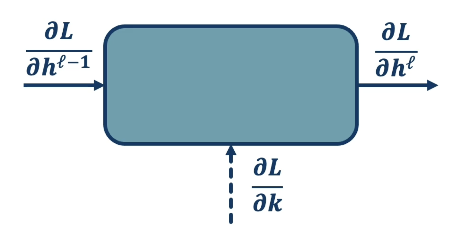
As with any other layer, assume we have access to the upstream gradient $\frac{\partial{L}}{\partial{h_{\ell}}}$ - the gradient of the loss w.r.t. our current layer’s output. As part of backpropagation, we are therefore interested in calculating…

1. Local Gradient w.r.t. Kernel $\frac{\partial{h_{\ell}}}{\partial{k}}$ to update our kernel weights, and
2. Local Gradient w.r.t. Input $\frac{\partial{h_{\ell}}}{\partial{h_{\ell - 1}}}$ to continue passing back the upstream gradient w.r.t. loss.

Gradient w.r.t. Kernel Weights#

How can we calculate the local gradient w.r.t. kernel weights $\frac{\partial{h_{\ell}}}{\partial{k}}$? This is a bit trickier than the case of a fully-connected layer, since we have sparse connectivity between inputs and outputs of the convolutional layer. Let’s simplify our problem by considering one kernel weight at a time. $\frac{\partial{h_{\ell}}}{\partial{k(a, b)}}; ~~~ a = k_h-1, ~ b = k_w-1$(for example, we can index each weight of a $3 \times 3$ kernel with $a = 2$ and $b = 2$)

How does any single kernel element $k(a, b)$ impact the output? Recall that the convolution operation involves striding the kernel across each valid receptive field of our input to generate the corresponding output node. At each receptive field, we have the following calculation (assume $h_{\ell} = Y$):

$Y_{(r,c)} = \sum_{a=0}^{k_h-1} \sum_{b=0}^{k_w - 1} X_{(r +a, ~c + b)}K_{(a, b)} + b$

Calculating the gradient for a single kernel weight relative to a single output node is trivial - we can expand the above formula to make this more clear. Assume we are interested in calculating the local gradient for kernel weight $K_{(0,0)}$ as part of the stride beginning at $X_{(0,0)}$.

$Y_{(0,0)} = X_{(0,0)} \times K_{(0, 0)} + \ldots + X_{(2, 2)} \times K_{(2, 2)} + b$

$\frac{\partial{Y_{(0,0)}}}{\partial{K_{(0,0)}}} = X_{(0,0)}$

We can then calculate the gradient of the loss by applying the chain rule through the relevant output node $Y_{(0,0)}$.

$\frac{\partial{L}}{\partial{K_{(0,0)}}} = \frac{\partial{L}}{\partial{Y_{(0,0)}}} \times \frac{\partial{Y_{(0,0)}}}{\partial{K_{(0,0)}}}$

Awesome! Now we’re done, right? Nope - this computation only considers a single path from the kernel weight to our final loss value (i.e., single receptive field $\rightarrow$ single input : kernel overlap $\rightarrow$ single output node). We should take the sum over all possible receptive fields to calculate our final partial derivative of loss w.r.t. kernel weight.

$\frac{\partial{L}}{\partial{K_{(0,0)}}} = \sum_{r=0}^{R}\sum_{c=0}^{C} \frac{\partial{L}}{\partial{Y_{(r,c)}}} \times \frac{\partial{Y_{(r,c)}}}{\partial{K_{(0,0)}}}$

We can generalize this computation to apply to any kernel weight $K_{(a,b)}$ to calculate the gradient of loss w.r.t. each kernel weight.

$\frac{\partial{L}}{\partial{K_{(a,b)}}} = \sum_{r=0}^{R}\sum_{c=0}^{C} \frac{\partial{L}}{\partial{Y_{(r,c)}}} \times \frac{\partial{Y_{(r,c)}}}{\partial{K_{(a,b)}}}$

Gradient w.r.t. Convolutional Input#

How can we continue passing our gradient $\frac{\partial{L}}{\partial{h_{\ell}}}$ backwards through a convolutional layer? We must calculate the local gradient w.r.t. the convolutional input $\frac{\partial h_{\ell}}{\partial{X}}$. Note that each input pixel $X(r,c)$ impacts the output $Y$ wherever it is part of a receptive field (and that each receptive field corresponds to a particular output node $Y_{(r,c)}$). In the case of $Y_{(0,0)}$ and $X_{(0,0)}$, we have…

$Y_{(0,0)} = X_{(0,0)} \times K_{(0, 0)} + \ldots + X_{(2, 2)} \times K_{(2, 2)} + b$

$\frac{\partial{Y_{(0,0)}}}{\partial{X_{(0,0)}}} = K_{(0,0)}$

To calculate the gradient of the loss function w.r.t. our input $X_{(0,0)}$, we must sum over each possible path from $X_{(0,0)}$ to the final loss. This translates to summing over each output node $Y_{(r,c)}$ where $X_{(0,0)}$ has involvement.

$\frac{\partial{L}}{\partial{X_{(r',c')}}} = \sum_{r=0}^{R}\sum_{c=0}^{C} \frac{\partial{L}}{\partial{Y_{(r,c)}}} \times \frac{\partial{Y_{(r,c)}}}{\partial{X_{(r',c')}}}$

Gradient Considerations for Pooling Layers#

Although pooling layers do not contain any learned parameters, we must still propagate our loss backwards through them to learn in earlier layers of the network. How can we calculate the gradient of the loss function w.r.t. inputs of a pooling layer?

Our gradient calculation depends on the pooling operation:

• Max Pooling: calculate local gradient $\frac{\partial{h_{\ell}}}{\partial{X}}$ as $1$ if $X_{(r,c)}$ is maximum for given output node, and $0$ otherwise.

  • Consider the example where we are computing the max pooling result for $Y_{(0,0)}$ based on a $2\times2$ pooling kernel. Assume $X_{(0,0)}$ is the maximum.

  $Y_{(0,0)} = \max(X_{(0, 0)}, X_{(0, 1)}, X_{(1, 0)}, X_{(1, 1)}) = X_{(0,0)}$

  $Y_{(0,0)} = X_{(0,0)} \rightarrow \frac{\partial{Y_{(0,0)}}}{\partial{X_{(0,0)}}} = 1$

• Average Pooling: calculate local gradient $\frac{\partial{h_{\ell}}}{\partial{X}}$ as $\frac{1}{N}$ for all $X$ involved in given output node.

  $Y_{(0,0)} = \frac{1}{N}(X_{(0, 0)} + X_{(0, 1)} + X_{(1, 0)} + X_{(1, 1)})$

  $\frac{\partial{Y_{(0,0)}}}{\partial{X_{(0,0)}}} = \frac{1}{N}$

In the case of any pooling operation, if we have overlapping receptive fields which result in an input being used for multiple different output nodes, we simply sum the gradients for each path to yield the final gradient.

CNN Architectures#

Recall that Neural Architecture refers to the composition of layers within a neural network, both in terms of arrangement and layer type. Given that we are familiar with a number of layer types (ex: linear, activation, convolutional, pooling, batch norm, etc.), what are some common architectural choices for arranging these layers into full-scale neural networks?

Simple CNN Architectures#

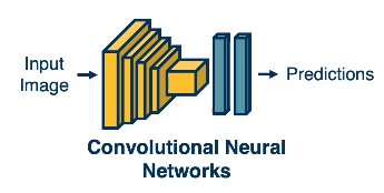
A simple CNN might first apply convolution + pooling layers to an input to extract spatially-focused features, then flatten the intermediate output and use linear transformations to map to output dimensionality. For example…

• Layer 1: Input (image)
• Layer 2: Convolution + Activation (e.g., ReLU)
• Layer 3: Max Pooling
• Layer 4: Convolution + Activation
• Layer 5: Flatten + Linear
• Layer 6: Softmax

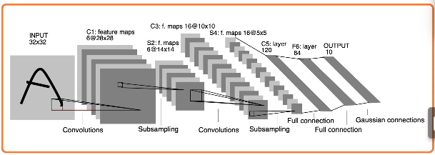
CNN implementations typically reduce the size of the kernel with each convolution, but increase the depth of the output via a larger number of kernels. For example…

One of the earliest CNNs was LeNet, developed by Yann LeCun and colleagues at Bell Labs (AT&T) in the late 1980s. The LeNet architecture involves a series of alternating convolutions + pooling layers, and concludes with a series of fully-connected layers.

Advanced CNN Architectures#

So what architectures are considered state-of-the-art (SoTA) for modern computer vision tasks? In order to discuss cutting-edge architectures, we should first establish an evaluation framework for their comparison.

A Benchmark Dataset is a standardized dataset used to evaluate and compare the performance of machine learning models. Benchmark datasets are usually specific to the machine learning task; for example, ImageNet is a benchmark dataset used to evaluate image classification models. ImageNet consists of 1.2 million labeled training examples, with a total of 1,000 output class categories. Advanced CNNs were first applied to ImageNet around 2012, and completely blew other approaches (such as SVCs) out of the water. As optimization / regularization / data augmentation approaches improved since 2012, so did CNN performance on the ImageNet dataset.

Unfortunately, we are unable to explore the infinite hypothesis space of possible CNN architectures. However, we can consider some of the best-performing advanced architectures that have emerged over the years:

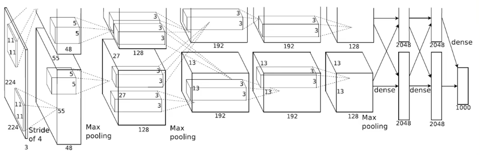
• AlexNet (2012): groundbreaking CNN created by Alex Krizhevsky, Ilya Sutskever, and Geoffrey Hinton.
  • Defining Characteristics: massive number of parameters; used ReLU instead of sigmoid.
  • Architecture: convolution $\rightarrow$ pooling $\rightarrow$ batch norm repeats, followed by linear layers.

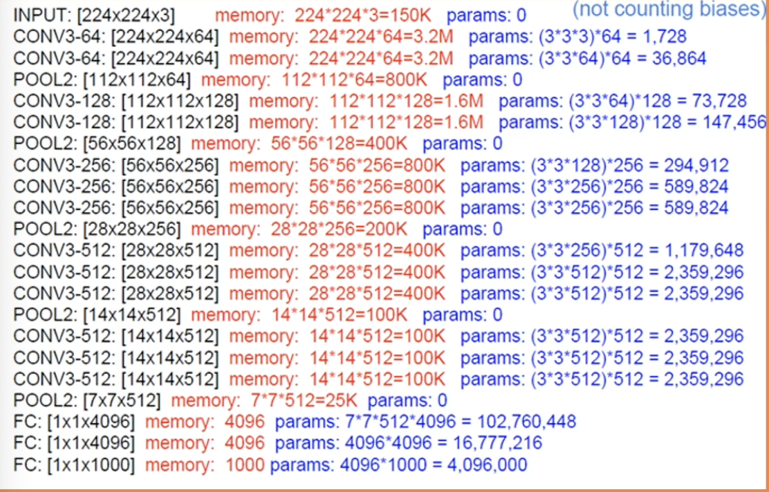
• VGG (2014): created by the Visual Geometry Group @ Oxford University.
  • Defining Characteristics: repeated “blocks” of sequential convolutional layers (ex: CONV3 $\rightarrow$ CONV3 $\rightarrow$ CONV3, with 3 being the kernel size). Deeper versions of VGG (ex: VGG-19) have more blocks.
  • Architecture: convolutional blocks separated by pooling layers, with final series of linear layers.

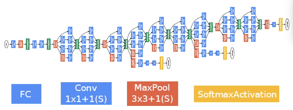
• Inception (2014): introduced by researchers at Google in 2014 as GoogLeNet.
  • Defining Characteristics: similar repeated block structure to VGG, but MUCH deeper; uses multi-scale feature maps, meaning feature maps of different sizes are extracted at each convolutional layer.
  • Architecture: parallel convolutional blocks separated by pooling layers, with final fully-connected layer.

Notice that advancements in CNN performance tend to correspond to deeper networks. This trend isn’t completely foolproof, since we eventually reach a point where we are no able to efficiently optimize model parameters. This leads CNNs with very high depth to perform similarly to those with much lower depths. In other words, optimization became a bottleneck for deep CNN performance.

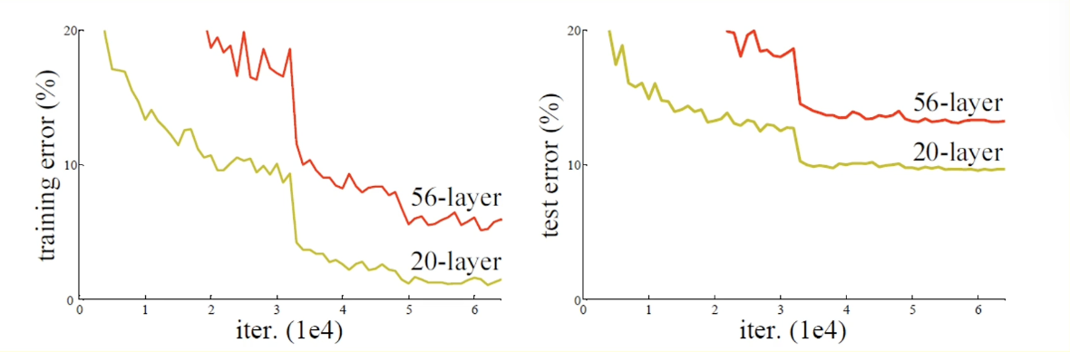
This issue spurred the innovation of Residual Connections - identity function connections that skip over portions of a neural network to improve gradient flow.

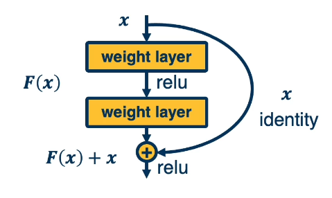
Residual connections are the basis of Residual Neural Networks such as ResNet-32 and ResNet-50. They allow deeper neural networks to learn much more effectively.

Transfer Learning and Generalization#

Generalization#

Given a machine learning algorithm, there are many sources of error that prevent our representation from being 1

• Optimization Error: optimization algorithm may not be able to identify the best set of weights for a given model, even if the model is perfect.
• Estimation Error: limited generalization from training model to test situations.
• Modeling Error: hypothesis space for model class does not include the true target function.

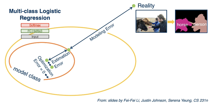
Overall, Generalization refers to a machine learning model’s ability to make accurate predictions on data not used for training. Each of the above sources of error may prevent a model from generalizing properly.

Transfer Learning#

In some situations, we might not have sufficient data to train a deep learning model for our problem. We can apply Transfer Learning to re-use a pre-trained neural network for a new application. Transfer learning works as follows:

• Step 1: Train a neural network on a large-scale dataset (ex: ImageNet).
• Step 2: Take your custom data and initialize the network with weights trained in Step 1.
  • Remove the last layer of the network corresponding to dataset-specific outputs.
  • Replace it with a new output layer specific to your task.
• Step 3: Continue training (with the new output layer) on your custom dataset.
  • Either fine-tune by updating all parameters, or freeze certain hidden layers / only update the output layer.

The key idea behind transfer learning is that features learned for one task might also be useful for another task. In other words, the parameter values of a trained neural network - which represent learned feature extractors - may be transferable from source to target task. Generalization quality is typically dependent on task type (ex: object recognition / classification). For example, if the target task is very different from the source task, transfer learning probably won’t work very well.

(all images obtained from Georgia Tech DL course materials)