Markov Decision Processes

Review of Machine Learning#

Recall that Machine Learning is the study of algorithms which learn from experience. There are three primary subfields of machine learning, distinguished by problem type.

• Supervised Learning: function approximation. Primary goal is to learn the functional mapping from inputs $X$ to outputs $y$.

  $f: X \rightarrow y$

• Unsupervised Learning: data description. Primary goal is to learn about the structure of unlabeled data $X$. This may involve tasks such as dimensionality reduction, clustering, and anomaly detection.

  $f : X$

• Reinforcement Learning: reward maximization. Primary goal is to learn optimal policy mapping environmental states to agent actions.

  $\pi: s \rightarrow a$

Introduction to Reinforcement Learning#

According to Wikipedia, Reinforcement Learning (RL) is concerned with how an intelligent agent should take actions in a dynamic environment to maximize a reward signal.

Grid World#

The most basic example of reinforcement learning is Grid World. We are given an environment represented by a grid. The grid contains some starting state, goal state, and penalty state(s). An agent is placed into the environment at the starting state, and may select one of four actions: up, down, left, or right.

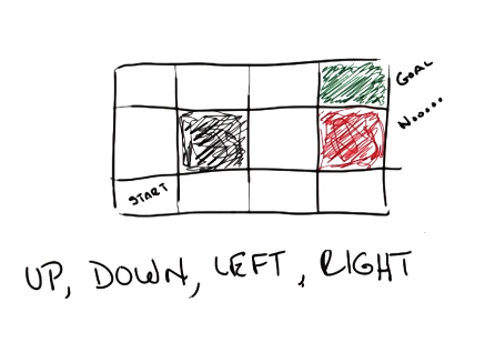
We introduce stochasticity into this process such that an agent’s action does not always result in the desired outcome.

$\Pr(A): \begin{cases} \text{correct action executes}& 0.8 \\ \text{action} ~ 90^o ~ \text{to the left executes} & 0.1 \\ \text{action} ~ 90^o ~ \text{to the right executes} & 0.1 \end{cases}$

Additionally, we define our reward function such that reaching the goal state is highly desirable, any intermediate state is mildly bad, and the penalty state is highly unfavorable.

$R(S): \begin{cases} \text{Goal} & +1 \\ \text{Penalty} & -1 \\ \text{Start} & 0 \\ \text{Other} & -0.04 \end{cases}$

Given this framework, we define the optimal mapping from states to actions as follows.

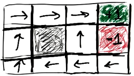
How did we come up with this solution? First, we need to define our reinforcement learning problem in more concrete terms.

Markov Decision Process#

A Markov Decision Process (MDP) is a formal mathematical representation of a reinforcement learning problem. MDPs capture problems such as Grid World by defining the following components:

• State Space $s \in S$ $\rightarrow$ set of possible environmental states attainable as part of the problem.
• Action Space $a \in A$ $\rightarrow$ set of possible actions an agent may take. May be restricted depending on the current environmental state $A(s)$.
• Model $T(s, a, s') \sim \Pr(s' \| s, a)$ $\rightarrow$ state transition matrix. Defines probability distribution of state transitions, therefore capturing stochasticity. Essentially the “physics” of the world.
  • In a fully deterministic world, transitions are not uncertain. However, this model still describes possible state transitions (i.e., $\Pr(s'\|s, a) \in \begin{Bmatrix} 0 & 1 \end{Bmatrix}$).
• Reward $R(s)$ $\rightarrow$ scalar value for being in a certain state. May also be defined relative to action $R(s, a)$ or previous state $R(s, a, s')$, depending on the formulation of the MDP.

There are a few key assumptions built into MDPs:

• MDPs are built on the Markov Property, which specifies that any state transition only depends on the previous state. This implies we do not define terms such as $\Pr(s_k \|s_0, \ldots, s_{k-1}, a)$ in the state transition matrix.
• The state transition matrix is assumed to have the same structure regardless of time. In other words, there is no deviation in the statistical properties of the state transition matrix over time. We therefore describe the state transition matrix as stationary.

Given this problem framework, the solution to any MDP is a Policy. A valid policy is a mapping from every possible environmental state to an action. This serves as a form of “lookup” for the agent while navigating through the MDP. The optimal policy for an MDP maximizes long-term reward.

$\pi(s) = a ~~~~~~~~~~~~~ \text{Optimal Policy}: ~\pi^*$

Considerations#

Credit Assignment#

One key problem of reinforcement learning as described so far is Temporal Credit Assignment. Given a delayed reward (such as reaching the end of Grid World or winning a chess game), how can we assign credit to actions taken over the course of an MDP trial?

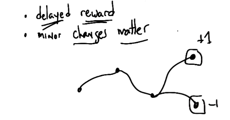
This formulation is in contrast to supervised learning, where every state would have a correct action with immediate “reward” (e.g., whether the predicted action is correct).

Sensitivity to Reward Structure#

Furthermore, our definition of rewards has major impact on optimal policy. For example, if we redefine the reward for “other” states as part of our aforementioned Grid World problem, we see very different optimal policies.

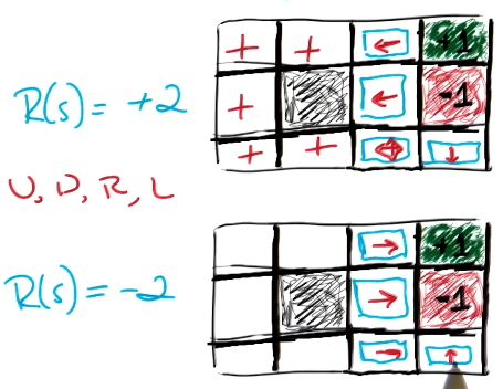
Since the reward function is often subjectively set by an MDP designer, it should utilize domain knowledge to target behaviors that would be desirable as part of the problem.

Time#

Our problem as described thus far has assumed infinite horizons, meaning the agent has an infinite number of time steps at their disposal. This is not common in practice - often times, real-world problems imply finite time. Note that the optimal policy can change depending on the number of available time steps.

$\text{Infinite Horizons}: ~~~ \pi(s) = a$

$\text{Finite Horizons}: ~~~\pi(s, t) = a$

Sequences of Rewards#

Additionally, we have discussed reward in the context of a single state. We can describe the utility of a sequence $V$ as the combined reward over a sequence of states.

$V(S_0, S_1, S_2) \in \mathbb{R}^{1}$

Given we have two sequences beginning in the same state $S_0$, and one sequence has greater utility than the other, we can draw the following conclusion.

\text{if} ~~ V(S_0, S_1, S_2, \ldots) > V(S_0, S_{1'}, S_{2'}, \ldots) \tag{1}

\text{then} ~~~ V(S_1, S_2, \ldots) > V(S_{1'}, S_{2'}, \ldots) \tag{2}

Okay, so how do we define “combined reward over a sequence of states”? Let’s try simply adding rewards across states.

$V(S_0, S_1, S_2, \ldots) = \sum_t R(S_t)$

The key problem with this representation is that, given infinite horizons and only positive reward, we will have infinite reward! In this case, we would not be able to compare two sequences.

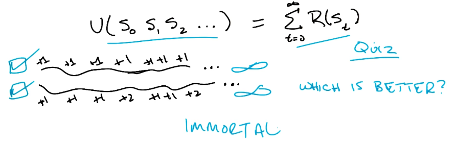
Instead, a better representation is to define the utility of a sequence as the discounted sum of rewards corresponding to individual states.

$V(S_0, S_1, S_2, \ldots) = \sum_t \gamma^{t} R(S_t) ~~~~~~~~~~ \gamma \in [0, 1)$

This is a geometric series, meaning we can define an upper bound on the result. Therefore, we can define a finite result even for an infinite sequence!

$\sum_t \gamma^t R(S_t) \leq (\sum_t \gamma^t) \times R_{MAX} = \frac{R_{MAX}}{1 - \gamma}$

Solving MDPs#

Defining the Optimal Policy#

Given our definition for the utility of a sequence of states, we can now more concretely define the optimal policy for an MDP.

$\pi^{*} = \arg \max_\pi \mathbb{E} \left[ \sum_t \gamma^t R(S_t) | \pi \right]$

Additionally, we define the utility of a state as the discounted sum of rewards over future states, given some policy for selecting actions to navigate through the state space. Note that reward describes the immediate feedback for entering a state, whereas utility describes long-term feedback over a sequence of states stemming from a given state.

$V^{\pi}(s) = \mathbb{E} \left[ \sum_t \gamma^t R(S_t) | \pi, S_0 = s \right]$

We can now rewrite our optimal policy in terms of utility. Assume utility is defined in terms of the optimal policy.

$\pi^{*}(s) = \arg \max_a \sum_{s'} T(s, a, s') V(s')$

Bellman Equation#

The Bellman Equation unrolls our utility function one level and incorporates concepts from our definition of optimal policy. The primary purpose of the Bellman Equation is to provide a solvable representation of state value.

$V(s) = R(s) + \gamma \max_a \sum_{s'} T(s, a, s') V(s')$

Note that a key characteristic of the Bellman Equation is recursion, since the function references itself within its definition!

Value Iteration#

Value Iteration is a specific algorithm which solves for state values using the Bellman Equation. More specifically, value iteration iteratively updates the state-value function $V(s)$ until convergence.

1. Initialize state utility $V(s)$ to random values.
2. LOOP (until convergence):
     - Iterate over states, updating state values based on current state values.

$\hat{V}_{t+1}(s) = R(s) + \gamma \max_a \sum_{s'} T(s, a, s') \hat{V}_t(s')$

Given the final converged utility function $\hat{V}(s)$, we define the optimal policy in terms of this function!

$\pi^{*}(s) = \arg \max_a \sum_{s'}T(s, a, s')\hat{V}(s')$

Note this algorithm requires us to define the reward function $R(s)$.

Policy Iteration#

As mentioned earlier, the goal of any MDP is to find the optimal policy mapping states to actions. Solving for state utility adds a level of computation - we first estimate state utility, then use our converged estimates of state utility to define policy. Is there any way we can skip over this intermediate computation to directly estimate the policy?

Policy Iteration is an alternative model-based approach to solving an MDP. Instead of iteratively estimating state value, policy iteration iteratively estimates the utility of a given policy.

1. Initialize state utility $V(s)$ to random values.
2. Initialize starting policy $\pi_0$ to a random guess.
3. LOOP (until convergence):
     - Evaluate: define state value $\hat{V}\_t(s)$ in terms of current policy $\pi_t$
     - Improve: compute new policy $\pi_{t+1}$ using new estimates for state value

$V_t(s) = R(s) + \gamma \sum_{s'} T(s, \pi_t(s), s') V_t(s')$

Policy iteration makes larger jumps, thereby tending to converge in fewer iterations than value iteration. However, each iteration of policy iteration is much more computationally expensive. This is because policy iteration involves solving a system of linear equations within the evaluation step, whereas value iteration is a sequence of simple updates.

(all images obtained from Georgia Tech ML course materials)