Reinforcement Learning

Intro to RL#

Machine Learning refers to the development of algorithms which learn from experience, rather than direct programming, to accomplish some task. Machine learning has three major subdivisions:

• Supervised Learning: function approximation. Learn functional mapping from input to output. $f : X \rightarrow Y$
• Unsupervised Learning: data description. Learn structures present in unlabeled data. $f(X)$
• Reinforcement Learning: reward maximization. Learn optimal policy to maximize reward. $\pi(s)$

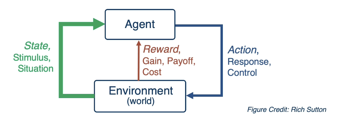
Reinforcement Learning (RL) involves sequential decision-making in an environment with evaluative feedback. As part of any RL system, an agent interacts with its environment to maximize some reward. The primary objective of the system is to learn the optimal policy mapping states of the environment to action choices.

Markov Decision Processes#

Definition + Components#

Markov Decision Processes (MDPs) provide a theoretical framework to represent RL problems by defining the following core components:

• $\mathcal{S}$: set of possible states.
• $\mathcal{A}$: set of possible actions.
• $\mathcal{R}(s, a, s')$: distribution of reward over possible state transitions.
• $\mathbb{T}(s, a, s')$: probabilistic state transition function.
• $\gamma$: discount factor.

The state transition function $\mathbb{T}$ defines the distribution over possible state transitions. For example, given a starting state $s$ and selected action $a$, what is the probability of reaching the end state $s'$? This is particularly important in the context of a stochastic environment.

The reward function assigns quantitative score to a tuple of $(s, a, s')$. As part of an MDP problem, we are ultimately interested in maximizing this score over a long-term period.

Given their definitions, these components are clearly crucial to any MDP framework! But guess what - in practice, we typically don’t know the true values for $\mathbb{T}$ nor $\mathcal{R}$. Instead, we simulate agent interactions with the environment to sample from the distributions, in order to estimate their values. However, for the purposes of this lesson, assume we have known $\mathbb{T}$ and $\mathcal{R}$ so we can focus on solving MDPs.

Solving MDPs#

In order to solve an MDP, we must find the optimal policy mapping states to actions.

• Deterministic Policy: $\pi(s) = a$
• Stochastic Policy: $\pi(a | s) = \Pr(A_t = a | S_t = s)$

A good policy maximizes the discounted sum of future rewards:

$\pi^{*} = \arg \max_{\pi} \mathbb{E} \left[ G_t | \pi \right]$

$G_t = R_{t+1} + \gamma R_{t+2} + \gamma^2 R_{t + 3} + \ldots = \sum_{k=0}^\infty\gamma^kR_{t+k+1}$

• State Value Function $V_{\pi}(s)$: expected return of being in state $s$ following policy $\pi$. Maps state to reward $V : S \rightarrow \mathbb{R}$. $V_{\pi}(s) = \mathbb{E}_{\pi} \left[ G_t | S_t = s \right]$
• State-Action Value Function $Q_{\pi}(s, a)$: expected return of taking action $a$ from state $s$ following policy $\pi$. Also known as the quality function. Maps state-action pair to reward $Q : S \times A \rightarrow \mathbb{R}$. $Q_{\pi}(s, a) = \mathbb{E}_{\pi} \left[G_t | S_t = s, A_t = a \right]$

Note that we can frame both the value function and optimal policy in terms of the quality function. More specifically…

• The optimal value of a state $V(s)$ is equivalent to the maximum state-action value $Q(s, a)$ over all possible actions.

$V^{*}(s) = \max_a Q^{*}(s, a)$

• The optimal policy at a given state $\pi(s)$ should select the action which maximizes state-action value $Q(s, a)$ over all possible actions.

$\pi^{*}(s) = \arg \max_a Q^{*}(s, a)$

The Bellman Optimality Equation is a recursive decomposition of our reward maximization problem into the immediate reward $R(s, a)$ and future expected reward.

$V^{*}(s) = \max_a \sum_{s'}^{ } \Pr(s' | s, a) [R(s, a) + \gamma V^{*}(s')]$

Given this equation, we can now estimate the state value function and state-action value function as follows:

• Value Iteration: initialize values for all states $V(s) = 0$. For each state, calculate $V^{i+1}(s) \leftarrow \max_a \sum_{s'}^{ } \Pr(s' | s, a) [R(s, a) + \gamma V^{i}(s')]$. Repeat until converging to $V^{*}(s)$.
• Q-Value Iteration: similar approach to value iteration, but loop over potential actions in addition to states. $Q^{i+1}(s, a) \leftarrow \sum_{s'}^{ } \Pr(s' | s, a) [R(s, a) + \gamma \max_{a'} Q^{i}(s', a')]$

For each of these approaches, we first estimate the value / quality function, then calculate the optimal policy via one walkthrough of greedy policy extraction. An alternative approach is to estimate value using a given policy, then update the policy based on value estimates - this is known as Policy Iteration.

$\pi_{i+1}(s) \leftarrow \arg \max_a \sum_{s'} \Pr(s' | s, a) [R(s, a) + \gamma V^{\pi_i}(s')]$

Value and Q-Value iteration are value-based approaches to solving MDPs. On the other hand, Policy Iteration is a policy-based method.

Example MDP: Grid World#

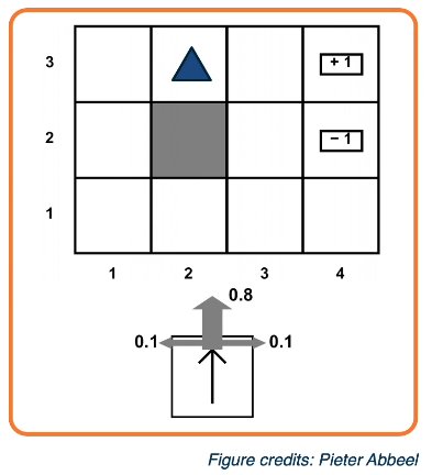
The most simple example of an RL system is Grid World which describes the following problem:

• Agent lives in a 2D grid environment.
• State: agent’s 2D coordinates.
• Actions: N, S, E, W.
• Rewards: +1/-1 at absorbing states.
• Stochastic State Transitions: 80% chance of proceeding in selected direction. 20% chance of proceeding perpendicular to selected direction (10% left, 10% right).

Deep Q-Learning#

Alright, so that’s all of reinforcement learning! Right? Not even close. One key issue with our current approach is the time complexity. Direct calculation of the state value function / state-action value function / policy has an unfavorable time complexity:

$\mathcal{O}(|\mathcal{S}|^2|\mathcal{A}|)$

In a simple example such as Grid World, this isn’t too bad. However, for even moderately complicated environments involving larger state and action spaces, these approaches become too computationally expensive. So what’s the solution?

Deep Q-Learning is an approach to solving MDPs which learns a parameterized Q-function to estimate the state-action value function. Given a state : action pair as input, the Q-function outputs a score. In the simplest case, we can use a linear model to represent our Q-function:

$Q(s, a; w, b) = w_a^{T}s + b_a$

In practice, we typically choose to fit a Deep Q-Network (DQN) to represent our Q-function. DQNs are simply neural networks which approximate the Q-function $Q(s, a)$.

Training a DQN#

So how does the learning process work? Recall that the Bellman Equation defines the Q-function as follows:

$Q^{*}(s, a) = \mathbb{E} \left[R(s, a) + \gamma \max_{a'} Q^{*}(s', a') \right]$

Our objective function - Temporal Difference (TD) Error - minimizes the difference between our predicted and TD target Q values. Note the TD target is calculated by taking the actual reward received $r$ and adding it to the discounted state-action value for the next state $s'$.

$\text{MSE Loss:} ~~ (Q(s, a) - (r + \max_{a'} \gamma Q(s', a')))^2$

There is one key issue with this representation - during parameter updates to $Q(s, a)$, the network is also changing its estimate of the TD target, thus “moving the goalposts” for the loss calculation. To solve this problem, DQNs introduce the Target Network as a separate, frozen copy of the network which is used to calculate the TD target. We may then update this frozen network at fixed intervals.

Gathering Data#

Given our optimization approach, how should we go about collecting data via agent experience with the environment?

1. We might start with a random data gathering policy $\pi_{\text{gather}}$ to collect instances of $(s, a, s', r)$.
2. Use the data to train our DQN, then use the DQN to update our policy $\pi_{\text{trained}}$.
3. Repeat this process until policy convergence.

While this approach is reasonable, it is problematic for one key reason - we are only exploring states which yield high reward relative to the current data-gathering policy. States with low reward as estimated by the current Q-function (but perhaps with high long-term reward) will be passed over. We must effectively balance Exploration vs. Exploitation by ensuring our algorithm strays from its path to explore alternative (lower-reward) paths:

• Exploration: select action that corresponds to uncertain rewards.
• Exploitation: select safe action that has good rewards according to the current Q-function.

Exploration vs. Exploitation efforts typically result in an Epsilon-Greedy approach to action selection. In practice, we use annealing to decay epsilon over time, which implies less weight is given to random action selection with increased experience.

$a_t = \begin{cases} \arg \max_a Q(s, a) & \text{with probability} ~ 1 - \epsilon \\ \text{random action} & \text{with probability} ~ \epsilon \end{cases}$

Policy-Based Methods#

Whereas value-based methods estimate state value to optimize the policy, policy-based methods focus on directly optimizing the policy itself.

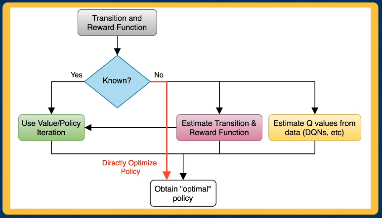
Similar to the case where we have a parameterized value function (as in DQN), we can also parameterize our policy.

$\pi_{\theta}(a|s) : \mathcal{S} \rightarrow \mathcal{A}$

Our objective function the expectation of discounted rewards over time.

$J(\theta) = \mathbb{E} \left[ \sum_{t=1}^T R(s_t, a_t) \right]$

Policy Gradients#

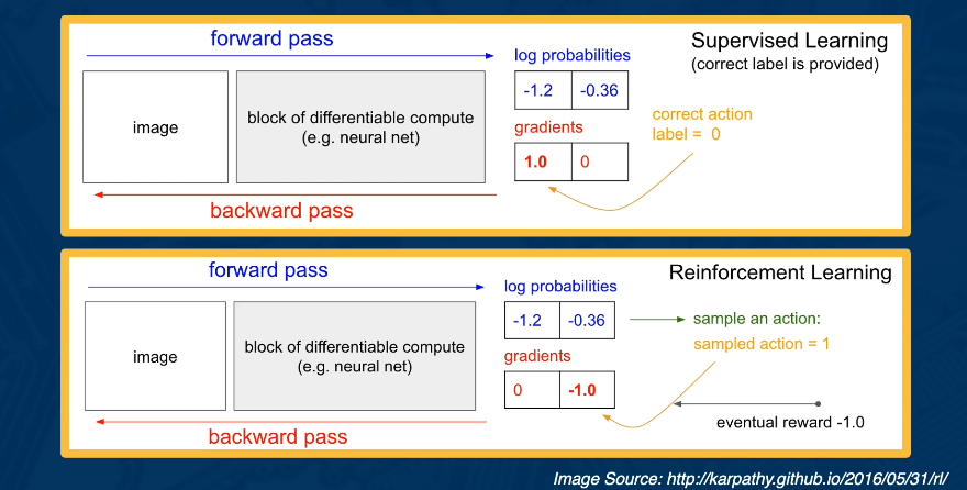
Given our objective, can we define the policy gradient to calculate during any update step of gradient descent? We define a similar setup to the case of supervised learning, but define our label as a sampled action.

(all images obtained from Georgia Tech DL course materials)