Model Training, Tuning, and Evaluation

Introduction#

In the previous section, we reviewed various machine learning (ML) algorithms built into the AWS SageMaker platform. However, most modern approaches require custom-built approaches built on neural networks. This section provides an overview of deep learning, neural network training & evaluation, and the integration of neural techniques with SageMaker.

Deep Learning#

Deep Learning is a subfield of machine learning concerned with deep neural networks, where depth refers to the number of hidden layers within the network.

History of Neural Networks#

An (artificial) Neural Network is a mathematical model organized as a series of layers / matrix transformations connected via non-linear activation functions. Neural networks have extreme representational power, extending far beyond the limits of most classical machine learning algorithms.

The first artificial neuron was introduced in 1943 via the McCulloch-Pitts Neuron, which computes basic boolean logic functions by multiplying binary inputs with weights.

Image Source

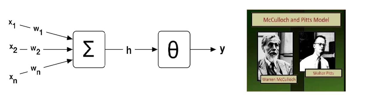
This idea was extended by Frank Rosenblatt in 1957 via the Perceptron, which was the first machine learning algorithm designed for artificial neurons. The perceptron defines a system in which continuous inputs are multiplied by learned weights (parameters) to produce a weighted sum, which is passed through an activation function to produce the final binary output.

Image Source

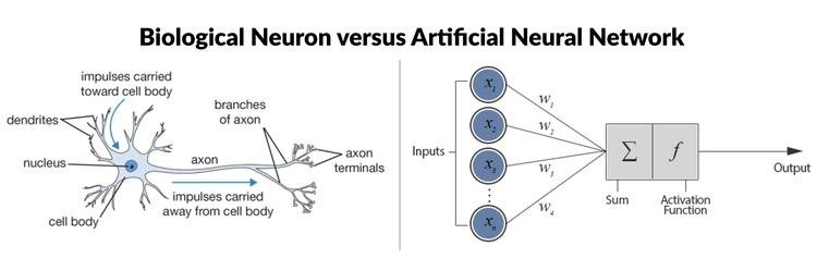
Chaining multiple perceptrons together produces a Multi-Layer Perceptron (MLP), which is a basic type of modern neural network.

Activation Functions#

An activation function processes the intermediate output (e.g., weighted sum) corresponding to a single layer within a neural network. There are many types of activation functions:

• Linear: $f(x) = x$
  • Not very useful in practice, since a weighted sum of weighted sums reduces to a single cumulative linear model.
  • Non-linear activation functions enable more complex learning.
• Binary: $f(x) = 1 ~ \text{if} ~ \sum_i x_iw_i > t, ~ 0 ~ \text{otherwise}$
  • Simple step function gating input via threshold $t$.
  • Incompatible with backpropagation due to non-differentiability.
• Sigmoid / Logistic: $f(x) = \frac{1}{1 + e^{-x}}$
  • Scales output to continuous range between 0 and 1.
  • Particularly susceptible to the vanishing gradient problem (discussed later).
• Tanh: $f(x) = \frac{sinh(x)}{cosh(x)} = \frac{e^x - e^{-x}}{e^x + e^{-x}}$
  • Scales output to continuous range between -1 and 1.
  • Suffers from issues with computational complexity.
• Rectified Linear Unit (ReLU): $f(x) = x ~ \text{if} ~ x > 0, ~ 0 ~ \text{otherwise}$
  • Easy and fast to compute.
  • Dying ReLU problem describes hindered learning when neurons receive consistent negative pre-activations.
• Leaky ReLU: $f(x) = x ~ \text{if} ~ x \geq 0, ~ \alpha \times x ~ \text{otherwise}$
  • Uses scaling factor $\alpha$ to reduce signal once weighted sum falls below threshold.
  • Scaling factor is learned in the case of parametric ReLU; set to constant value for leaky ReLU.
  • Solves dying ReLU problem at the cost of increased computational complexity.
• Softmax: $f(x) = \begin{bmatrix}\frac{e^{x_k}}{\sum_z e^{x_z}} ~ \text{for} ~ k ~ \text{in} ~ \text{n classes} \end{bmatrix}$
  • Used as the final output layer for multi-class classification problems. Conceptually, converts raw outputs to probabilities for each class label.
  • Sigmoid is a special case of Softmax.

In general, we tend to start with ReLU then try Leaky ReLU / PReLU for more advanced problems. Multi-class classification problems require Softmax, and RNNs tend to perform well with Tanh.

CNNs#

A Convolutional Neural Network (CNN) is a specific type of neural architecture which builds on the mathematical convolution operation (blends two functions by sliding, reversing, and multiplying them together). $(f * g)(t) = \int_{-\infty}^{\infty} f(\tau) g(t - \tau) d\tau$ By sliding one function along another, we define a feature-location invariant model. This is particularly efficient in the case of image data, where features used to process input pixels are shared across the entire image!

In the context of image data, CNNs slide a learned matrix of weights (referred to as a kernel) across an image, taking the weighted sum of pixels within the current receptive field of the image. Each position in the output matrix corresponds to a weighted sum of kernel $\times$ receptive field. This enables CNNs to scan an entire image and produce location-aware output.

Within a CNN, convolutional layers are responsible for performing the actual convolution operation. Lower-level math is abstracted away in modern deep learning libraries (e.g., Conv2D in TensorFlow). Other common CNN layer types include:

• Pooling Layers: reduce the dimensionality of multi-dimensional layers by summarizing regions of the input (ex: max over regions of an input 2D matrix).
• Flatten Layers: convert multi-dimensional layers (ex: 2D convolutional output) into 1D. Often used to preprocess the output of convolutional layers prior to standard linear layers.

Data dimensionality is particularly tricky when dealing with CNNs. Ensure that your source data is of the appropriate dimensionality (e.g., $\text{width} \times \text{length} \times \text{color channels}$), and define weight matrices for layers by considering the dimensionality of previous-layer output.

The amount of possible CNN architectures (layers, layer types, neurons within each layer, and activation functions) is unfathomable! Fortunately, researchers have defined specialized CNN architectures well-suited for particular applications.

• LeNet-5: handwriting recognition.
• AlexNet: image classification.
• GoogLeNet: defines inception modules as groupings of convolution layers.
• ResNet: residual network which greatly increases depth without cost to performance via skip connections.

RNNs#

A Recurrent Neural Network (RNN) uses the concept of recurrence to process sequence data. It carries information forward through the sequence by maintaining a hidden state. RNNs are used for analyzing time-series data, or data consisting of sequences of arbitrary length (e.g., text).

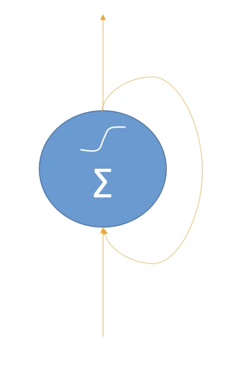
There are four major RNN topologies corresponding to different applications, mostly dependent on the types of input and output.

• Sequence-to-Sequence: given an input sequence, predicts an output sequence.
  • Ex: time-series prediction
• Sequence-to-Vector: given an input sequence, predicts an output vector (classification / regression).
  • Ex: sentiment analysis, text classification
• Vector-to-Sequence: given an input vector (e.g., encoded image), predicts an output sequence.
  • Ex: caption text generation for images
• Encoder-Decoder: given an input sequence, encoder produces an intermediate latent representation (vector) used as input for the decoder, which produces an output sequence.
  • Ex: machine translation, text generation

RNN training must account for hidden state from previous tokens - backpropagation through time unrolls recurrence by chaining backpropagation across time steps. Truncated backpropagation through time avoids issues with infeasible computational overhead.

Furthermore, RNNs have different structural motifs:

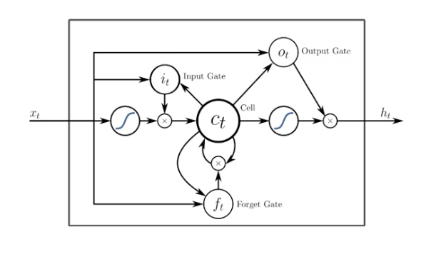
• Long Short-Term Memory (LSTM) Cell: maintains separate hidden states for short-term and long-term memory.
• Gated Recurrent Unit: simplified LSTM cell without major sacrifice to performance.

Training Neural Networks#

Neural network parameters are learned via Gradient Descent, which iteratively updates values using the gradient of the loss function w.r.t. parameters.

$w_{k+1} = w_k - \alpha \times \nabla_w L$

There are many different Hyperparameters for gradient descent, which serve as tunable configuration settings for a machine learning model other than directly learned parameters.

• Learning Rate: scaling factor used to control update size during any given step of gradient descent. $\alpha$ in the above equation.
• Epochs: an epoch is a single pass through the entire training dataset. Epoch count specifies the number of epochs for training.
• Batch Size: amount of instances used within a single iteration of stochastic gradient descent (SGD). We iterate over batches within any given epoch.

Note that batch size and learning rate have great impact on learning. Smaller batch sizes tend to avoid local minima, whereas large batch sizes may converge on the wrong solution at random. Larger learning rates may overshoot the correct solution, while smaller learning rates increase training time. Ultimately, the best values for these hyperparameters depend on the specific problem / dataset at hand, emphasizing the importance of Hyperparameter Tuning.

Regularization Techniques#

In the context of machine learning, Regularization refers to any technique intended to mitigate overfitting. Recall that overfitting refers to a model learning noisy patterns in the training data, which do not properly generalize to the pattern we are trying to represent. Overfitting is characterized by a large gap between training and validation (holdout) performance.

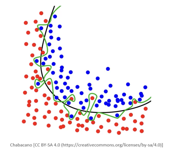
Common regularization techniques include:

• Reducing the complexity of the model (decrease hidden layers, neurons per hidden layer).
• Dropout Layer: randomly drops neurons within the layer during training. Forces neurons to learn an effective joint representation of the pattern, as opposed to relying heavily on any single neuron.
• Early Stopping: automatically stops training after some number of epochs without an improvement in validation accuracy. Requires training and validation data.

Certain regularization methods are based on penalty applied to the loss function during optimization.

• L1 Regularization: additional loss based on sum of absolute values for weights. $\lambda \times \sum_i |w_i|$
  • Sparse regularization
  • Performs feature selection $\rightarrow$ coefficients shrink to 0
• L2 Regularization: additional loss based on sum of squared weight values. $\lambda \times \sum_i w_i^2$
  • Dense regularization
  • All features remain in play

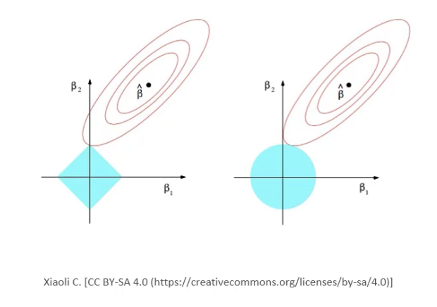
Lambda $\lambda$ is used as a scaling factor to control the impact of the penalty term on loss.

Common Training Issues#

Certain issues are common when training via gradient descent:

• Vanishing Gradient: gradient estimates approach zero.
• Exploding Gradient: gradient estimates become too large.

These issues may slow and/or completely prevent effective learning, as well as introduce numerical precision errors into the process. They are prevalent in the case of deep neural networks, since gradients are passed to earlier layers via the chain rule (multiplication of local gradients).

Certain activation functions (e.g., ReLU) and neural architectures (residual networks) are better suited to avoid these problems. Overall, gradient checking is a good diagnostic tool to ensure neural network training is successful.

Model Evaluation#

$\underline{\text{Classification Metrics}}$

A Confusion Matrix summarizes true positives / negatives and false positives / negatives. For example, a binary confusion matrix might be structured as follows.

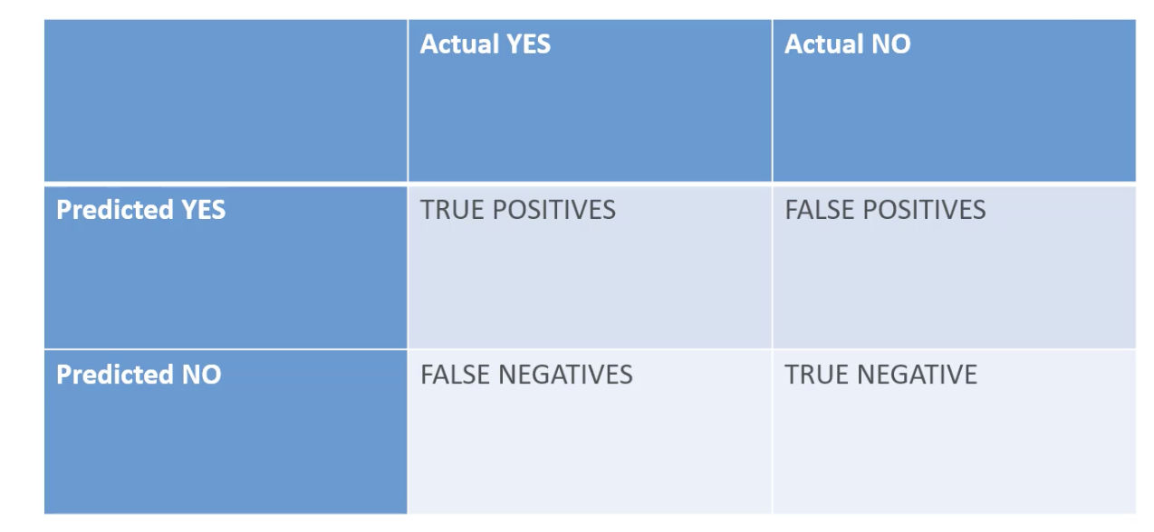
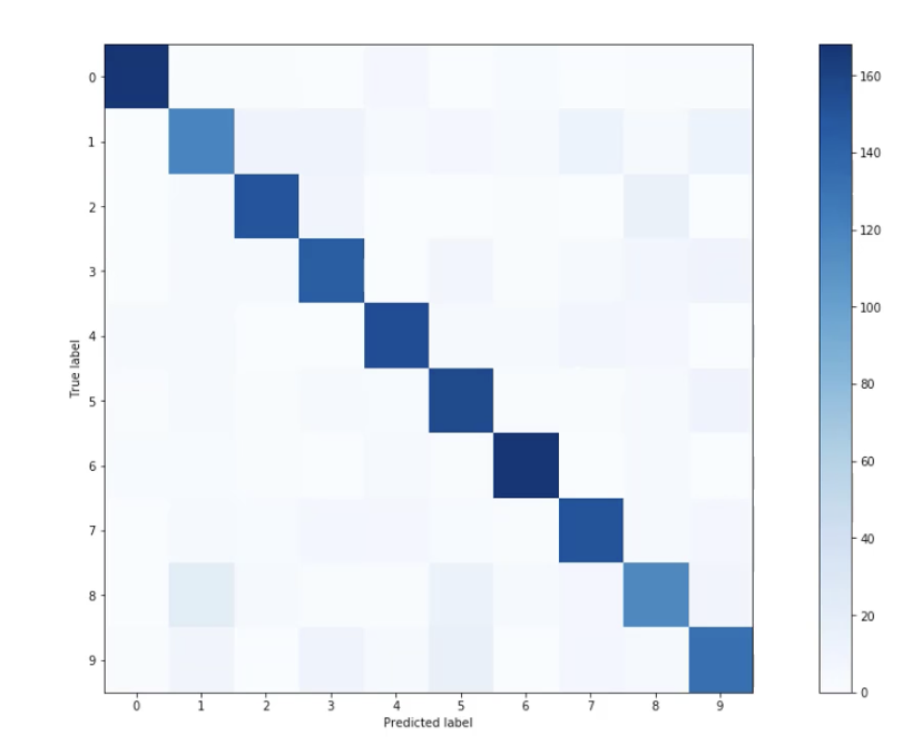
Multi-class confusion matrices generalize this concept to a $k \times k$ matrix, with $k$ representing the number of class labels.

Certain metrics are relevant in the context of binary classification:

• Accuracy: correct prediction rate. May be problematic to optimize over in the case of class imbalance. $\frac{\text{TP + TN}}{\text{TP + TN + FP + FN}}$
• Precision: predictive positive rate. Optimize to limit false positives. $\frac{\text{TP}}{\text{TP + FP}}$
• Recall: true positive detection rate. Optimize to limit false negatives. $\frac{\text{TP}}{\text{TP + FN}}$
• F1 Score: harmonic mean of precision and sensitivity. Optimize to balance benefits of precision and recall. $\frac{2 \times \text{TP}}{2 \times \text{TP + FP + FN}}$
• Receiver Operating Characteristic (ROC) Curve: plots true positive rate (recall) vs. false positive rate at various classification threshold values.
  • Area Under the Curve (AUC): probability that classifier ranks randomly chosen positive instance higher than randomly chosen negative instance.

Many of these metrics generalize to the multi-class setting by either 1) averaging over classes, or 2) considering a single class in isolation.

$\underline{\text{Regression Metrics}}$

R-Squared - otherwise known as the coefficient of determination - measures how well an independent variable explains the variance in a dependent variable. It represents the proportion of variance in the dependent variable that is predicted by the independent variable. We might apply R-squared in the context of regression by computing between observed and predicted values.

Other evaluation metrics for regression measure error between observed and predicted values:

• Mean Absolute Error: average absolute error between observed and predicted values. $\text{MAE} = \frac{1}{n} \sum_i | y_i - \hat{y_i} |$
• Root Mean Squared Error (RMSE): square root of average squared error between observed and predicted values. $\text{RMSE} = \sqrt{\frac{1}{n} \sum_i (y_i - \hat{y_i})^2}$

SageMaker Tools#

AMT and Hyperparameter Tuning#

Automatic Model Tuning (AMT) is a SageMaker service for performing hyperparameter tuning over specified ranges, relative to a specified optimization metric. It uses Bayesian optimization to intelligently explore hyperparameter combinations.

There are a few recommended practices for using AMT:

• Don’t optimize too many hyperparameters
• Limit ranges to as small as possible
• Use logarithmic scales for ranges when appropriate
• Don’t run too many training jobs in parallel; this limits the efficiency of Bayesian optimization learnings

AMT supports early stopping and warm start functionalities to improve tuning results. Additionally, the user may opt to use an alternative approach to Bayesian optimization, such as grid search or random search.

AutoML#

SageMaker Autopilot is a wrapper for AutoML. It enables automatic algorithm selection, preprocessing, hyperparameter tuning, and infrastructure provisioning.

Autopilot has a few built-in training modes:

• HPO: Hyperparameter Optimization
  • Selects algorithm most relevant to input dataset, and best range of hyperparameters.
  • Performs up to 100 trials of optimization to identify best hyperparameters.
    • Bayesian optimization for smaller datasets (< 100MB), multi-fidelity optimization for larger datasets.
• Ensembling
  • Trains multiple base models (tree-based, neural networks).
  • Performs 10 trials of hyperparameter search for each base model.
  • Combines base models using stacking ensemble method.
• Auto
  • HPO if input dataset is larger than 100MB (default).
  • Ensembling if input dataset is smaller than 100MB.

Autopilot also offers explainability by integrating with SageMaker Clarify. Feature attribution methods (ex: Shapley values) indicate which features are most important for a given prediction.

Model Registry#

The SageMaker Model Registry is a catalog for models, enabling users to manage their model versions and store associated metadata. Centralizing a library of models in one shared location enables easy and regulated access across an organization.

Integrations#

MLFlow is an open-source platform for machine learning and generative AI workflows. It offers useful features for all aspects of the ML process, including observability, evaluations, tracking, model management, and model deployment through the use of a tracking server. SageMaker offers a managed MLFlow tracking server to assist with experimentation.

SageMaker also integrates with Tensorboard to offer visualized model performance over the course of training. This is particularly useful for debugging issues with training, such as vanishing gradients, unstable learning, or overfitting.

(all information obtained from AWS Certified Machine Learning Engineer Associate: Hands On! course on Udemy)