Data Transformation, Integrity, and Feature Engineering

Introduction#

Following ingestion of input data for a machine learning project, it must be transformed and standardized to ensure compatibility with mathematical modeling. This section reviews common approaches and AWS services for data transformation.

EMR and Hadoop#

Elastic MapReduce is a managed Hadoop framework which runs on EC2 instances. EMR provides a method for distributing the processing load associated with heavy computational tasks, such as pre-processing massive datasets for machine learning training.

An EMR cluster consists of multiple collaborating EC2 instances, which are referred to as nodes.

Master Node: manages the cluster by coordinating tasks across instances. Single EC2 instance.
Core Node: hosts data and runs computations. Can be scaled up or down.
Task Node: runs computations, but does not host data. Can be scaled up or down. Good use of spot instances.

Transient EMR clusters automatically terminate after completing their tasks. Long-Running clusters continue to run and remain indefinitely available for computation.

EMR Serverless#

Serverless is a cloud computing framework in which the cloud provider managers the servers, and dynamically allocates instances as appropriate. EMR Serverless is therefore the same as EMR, but with AWS managing the underlying capacity of worker nodes.

Apache Hadoop and Spark#

Hadoop is a distributed computing framework built in layers:

Hadoop Distributed File System (HDFS): lowest level distributing data across instances of a cluster. Lost upon termination of the cluster, but useful for caching intermediate results.
Yet Another Resource Negotiator (YARN): large-scale distributed operating system for big data applications.
MapReduce: programming approach for splitting a large job into many parallel computations, then combining the results. Consists of mapper and reducer functions.

In the modern distributed computing landscape, Apache Spark has taken the place of MapReduce as a simpler service for distributed computing. Spark has APIs for common programming languages (Python, Scala, Java, R) offering many utilities:

Spark Streaming: enables scalable, high-throughput stream processing of live data streams (e.g., ingested from Apache Kafka / Kinesis).
Spark SQL: module for structured data processing using distributed collections of data, providing user with ability to execute SQL queries on distributed data.
MLlib: offers distributed computing interface for common machine learning algorithms (ex: classification, regression, clustering, etc.).
GraphX: distributed graph processing framework enabling ETL / graph computation at scale.

Data Transformation Methods#

Feature Engineering#

Feature Engineering refers to the manual derivation of new features, with the intention being to create more useful input features for model training.

"Applied machine learning is basically feature engineering."
- Andrew Ng

Why is feature engineering important in the first place? Couldn’t we simply derive an unbounded amount of features, and plug them all into our machine learning model? The Curse of Dimensionality describes how too many features can be problematic, since the amount of data required to generalize grows exponentially with the number of input dimensions (features).

Most of feature engineering involves using domain knowledge to select the features most relevant to the problem at hand. By limiting the set of input features to relevant predictors, we avoid sparse data (in high dimensionality) without sacrifice to model performance.

Imputing Missing Data#

Prior to training a machine learning model, we must ensure our input dataset does not contain missing values. Imputation is the process of filling missing values according to one of many potential strategies:

Mean Replacement: replace missing values with the average value from the rest of the column / feature. Fast and easy, but tends to provide low-quality estimates.
- Median Replacement may be more appropriate in the case of outliers.
- Only applies to numeric variables; Mode Replacement is the analogous approach for categorical variables.
Dropping Rows: exclude rows containing any missing value. Appropriate in the case of limited missing values, but may bias the training data.
ML-Based Imputation: apply machine learning model to impute missing data.
- KNN: average the feature values for the k most similar rows.
- Deep Learning: construct a DL model to predict the missing value based on other features; works very well fro categorical data.
- Regression: estimate linear / non-linear relationships between missing feature (outcome) and other features (predictors). Ex: Multiple Imputation by Chained Equations (MICE).

Perhaps the best way to fill missing values is to fix the problem at the source by increasing the quantity or improving the quality of input data.

Dealing with Imbalanced Data#

In the context of machine learning, an Imbalanced Dataset has an outcome variable with very different class proportions. For example, consider binary fraud as an outcome - the “positive” class is much less frequent than the “negative” class. This can skew our ML model to favor predicting the majority outcome, inflating accuracy but limiting model utility.

How can we deal with imbalanced data?

Oversampling: duplicate samples from the majority class at random.
Undersampling: remove samples from the minority class at random.
Synthetic Minority Over-sampling Technique (SMOTE): generates new samples of the minority class using nearest neighbors.
- Randomly select minority class sample.
- Run k-nearest neighbors.
- Create new synthetic minority class sample using mean of neighbors.

Handling Outliers#

Recall that Variance refers to the average of the squared differences from the mean. This estimates the relative spread of our data.

$\sigma^2 = \frac{\sum_i (x_i - \bar{x})^2}{n}$

Standard Deviation is the square root of variance, which places our measure of spread on the same scale as the original variable. Standard deviation is commonly used to identify outliers - for example, data points that lie more than one standard deviation from the mean may be considered unusual.

Given that we’ve identified outliers, how should we deal with them? Depending on the context, we may want to remove records with outliers from our training data.

Binning, Transforming, Encoding, Scaling, and Shuffling#

What other preprocessing steps should we apply to our input data?

Binning: bucket observations based on ranges of values. Transforms numeric data to ordinal data. This is especially useful when there is uncertainty in the original measurements.
Transforming: apply some function (ex: logarithm) to a feature, better suiting it for training.
Encoding: transform feature into format expected by model.
- Example: One-Hot Encoding transforms a categorical feature with k levels into k features with binary indicators, representing whether the given instance falls within this category level.
Scaling = Normalization: changes the scale / distribution of a feature to an expected range.
- Some models (ex: k-means) require features to be scaled to comparable values.
Shuffling: randomizes the order of instances in training data, preventing certain models from learning residual signals in the training data resulting from the order in which they were collected.
- Ex: reinforcement learning and replay buffer.

SageMaker AI#

SageMaker AI (previously SageMaker) is the AWS service dedicated to machine learning. It supports the entire machine learning lifecycle, including…

Data Gathering + Preprocessing: fetching the training data for ML modeling.
Model Training + Evaluation: training the ML model and evaluating its quality.
Model Deployment + Monitoring: deploying the trained ML model as a service and monitoring its performance in production.

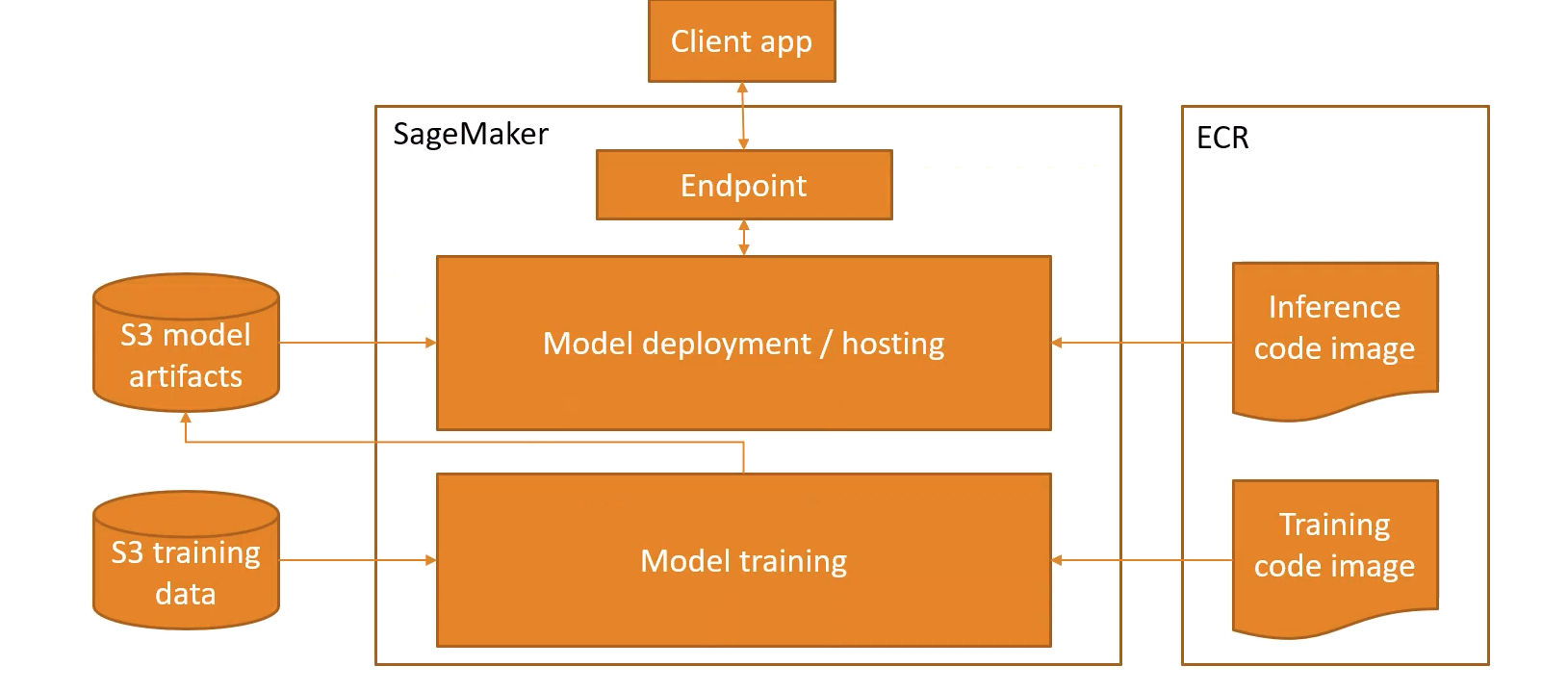
How does SageMaker AI work and integrate with other AWS tools?

S3: stores model artifacts and training data.
SageMaker: performs model training, saving model artifacts to S3. Exposes an endpoint where client applications may submit HTTP requests to gather prediction data.
ECR: defines images for inference code (model deployment + hosting) and training code (model training).
- ECR = Elastic Container Registry

SageMaker AI Domains#

The first step to using SageMaker AI is creating a domain. Domains organize users, applications, and resources as follows:

Shared EFS Volume for storage.
Authorized users for access.
Configuration settings (policy, VPC, etc.).

Any domain has two Virtual Private Cloud (VPC)‘s by default:

Internet Access: managed by SageMaker AI.
Domain VPC: encrypted traffic to EFS volume; user specifies VPC, subnets, and security groups.

Data Processing, Training, and Deployment#

Okay, so how do we use SageMaker AI to perform the typical steps required for a machine learning project?

STEP 1: Data Processing

Input data is typically stored on S3, but may be ingested from other AWS sources (ex: Athena, EMR, Redshift).
Set up a processing container (either provided by SageMaker AI or user-specified) to preprocess data and output it to S3.

STEP 2: Model Training

Create a training job in SageMaker AI. Requires URL of S3 bucket with training data, ML compute resources, URL of S3 bucket for output (model artifacts), and ECR path to training code.
Select a SageMaker AI training method, or specify your own via the training code.

STEP 3: Model Deployment

SageMaker AI supports two deployment options:
- Persistent Endpoint: makes individual predictions on-demand; always available.
- Batch Transform: retrieves predictions for an entire dataset at once.
SageMaker AI provides a number of other useful options:
- SageMaker Neo: supports model deployment to edge devices (ex: self-driving car).
- Automatic Scaling: increase / decrease # of endpoints as needed.

SageMaker Data Wrangler#

Data Wrangler is a visual interface for ETL integrated into SageMaker Studio, and is primarily used to prepare data for machine learning. It assists the user with code generation to match their specific needs for preprocessing. In addition to preprocessing, Data Wrangler provides basic tools for visualization and statistical analysis.

SageMaker Model Monitor#

Model Monitor is a tool offered through SageMaker AI which enables users to receive automated AWS CloudWatch alerts on quality deviations for deployed models. It offers functionality for…

Visualizing data drift or model drift.
Automatic detection of anomalies and outliers.
Detection of new features or feature attribution drift.

Whereas Model Monitor is a code-free service baked into SageMaker, other cloud and language-agnostic coding frameworks such as MLflow can be integrated with deployed models to support monitoring efforts.

SageMaker Feature Store#

In the context of machine learning, a feature is a particular column / variable of the input dataset. SageMaker Feature Store provides a centralized location for feature storage, enabling integration with many different models or services. It is compatible with both streaming and batch data loading options, and encrypts data at rest and in transit.

AWS Glue#

Glue is a serverless AWS system which 1) provides table definitions and schema to unstructured data (ex: S3 data lakes, RDS, etc.), and 2) enables custom event-driven ETL jobs on an Apache Spark cluster.

The Glue Crawler scans data in S3 to construct a schema (table definition, data types) for unstructured data. Once cataloged, this enables users to query unstructured data as if it were stored within a structured data warehouse. Glue provides the “glue” between the relational database interface and unstructured data lake without copying data into a data warehouse.

Tools within Glue#

Glue Studio is a visual (GUI) interface for setting up ETL workflows in Glue. The services offered by Glue Studio are very similar to those found in Azure Synapse Analytics pipelines. We define our data source(s), any transformations, and data target destionation(s) by creating a Directed Acyclic Graph (DAG) within Glue Studio’s visaul interface.

Glue Data Quality integrates into Glue jobs to monitor and detect aspects of data quality, including expected values / range / standard deviation for a given feature. Data quality alerts may terminate the job, or simply appear as log messages in CloudWatch.

Glue DataBrew is a visual data preparation tool used to preprocess large datasets. DataBrew serves the “transform” stage of an ETL process. The user creates “recipes” of transformations, which may be saved as jobs within a larger Glue project. How do we handle personally-identifiable information (PII) in DataBrew transformations?

Substitution: replace PII feature with random values.
Shuffling: recombine identifiers with PII feature such that the value is not associated with its original identifier.
Encryption: define transformed field as encrypted value of PII feature. Encryption may be deterministic or probabilistic.
Deletion: drop PII feature entirely.

Amazon Athena#

Athena is a serverless interactive query service for S3, enabling the user to utilize SQL queries with raw S3 data. Athena supports various data types (structured, unstructured, semi-structured), in addition to a wide range of data formats:

Human Readable: csv, tsv, JSON
Splittable (for parallelization): ORC, Parquet, Avro
Compressed: Snappy, Zlib, LZO, Gzip

How does Athena integrate with Glue? Any S3 bucket with a published Glue catalog is accessible via Athena.

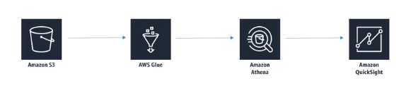
Athena defines workgroups to organize users / teams / apps / workloads to control query access, track costs, and define data limits. Workgroups integrate with IAM, CloudWatch, and SNS for data governance and monitoring capabilities.

At its core, Athena is a SQL query engine. It should not be utilized for highly formatted reports / data visualization (QuickSight) or pure ETL workloads (Glue).

CREATE TABLE AS SELECT and Performance#

Recall that all data queried through Athena is stored in its native format within Amazon S3. In the context of SQL, CREATE TABLE AS SELECT is used to create a new table from query results. When combined with Athena, this statement can be used to convert data into a new underlying format which may improve querying performance.

CREATE TABLE my_orc_ctas_table
WITH (
  external_location = 's3://my_athena_results/my_orc_ctas_table/', format='ORC'
) AS SELECT * FROM old_table;

Okay, so how do data formats influence performance in Athena? Athena tends to prefer columnar data (ORC, Parquet), and a small number of large files over a large number of small files.

ACID Transactions#

ACID is a set of properties for database transactions which guarantee data validity despite any errors or failures in the application.

Atomicity: an ACID transaction is treated as a single unit of work. If any stage of the transaction fails, any previously executed operations will roll back.
Consistency: each transaction is executed in an expected fashion and leaves the system in a consistent state.
Isolation: concurrent transactions submitted by multiple users will not interfere with each other.
Durability: any committed transaction is saved with permanent effects, even in the event of a system failure.