Randomized Optimization

What is Unsupervised Learning?#

Recall that Machine Learning (ML) is divided into three primary subfields:

• Supervised Learning: function approximation. Goal is to learn functional mapping from input $\mathbf{X}$ to output(s) $\mathbf{y}$.

$f(\mathbf{X}) = \mathbf{y}$

• Unsupervised Learning: data description. Goal is to learn something about the structure of the data $\mathbf{X}$, without regard for any particular output.

$f(\mathbf{X})$

• Reinforcement Learning: reward maximization. Goal is to learn an optimal policy mapping environmental states $s \in S$ to agent actions $a \in A(s)$ as to maximize long-term reward.

$\pi(s) = a ~~~ \forall s \in S$

We more concretely define Unsupervised Learning as a class of machine learning algorithms dedicated to analyzing unlabeled data. There are many types of unsupervised learning methods, with each type serving a different goal.

• Clustering $\rightarrow$ group instances by similarity into categories.
• Dimensionality Reduction $\rightarrow$ identify a more compact representation of the original data.

In this lesson, we will focus on randomized optimization techniques. Note that randomized optimization is a general class of computational methods, and is not typically considered a distinct subfield of unsupervised learning.

Randomized Optimization#

What is Optimization?#

Optimization refers to a general problem in which we seek to “find the best” value relative to a function of interest. We define the following components w.r.t. an optimization problem:

• Input Space $\mathbf{X}$: set of possible values our input can take on.
• Objective Function $f(\mathbf{X})$: scalar-valued function to be maximized (or minimized).

The goal of any optimization problem is therefore to find the input $\mathbf{x} \in \mathbf{X}$ which produces the best value of the objective function. This is analogous to an argmax or argmin depending on which direction is preferred.

General Approaches#

We can approach optimization in a few key ways - often our choice of optimization strategy depends on characteristics of the problem at hand.

• Manually Test: calculate output $f(\mathbf{x})$ over full input space $\mathbf{x} \in \mathbf{X}$. This is feasible in the case of a small input space, but not reasonable otherwise.
• Calculus: solve for optimum using principles of calculus (differentiation). This requires the objective function to have a solvable derivative, as well as a continuous input space.

What if these assumptions don’t hold? For example, consider a hypothetical problem with a large input space and complex function with no solvable derivative. Under these circumstances, we turn to Randomized Optimization (RO), which introduces stochasticity into the optimization process to improve search efficiency.

RO Methods#

Hill Climbing#

Hill Climbing is a basic RO algorithm which relies on the notion of proximity to iteratively optimize an objective function.

1. Randomly initialize input by selecting $\mathbf{x} \in \mathbf{X}$.
2. Loop indefinitely:

• Define neighbors to $\mathbf{x}$ as $\mathbf{n} \in \mathbf{N}$.
• Calculate output value $f(\mathbf{n})$ for each neighbor and current input $f(\mathbf{x})$.
• If: $f(\mathbf{n}) > f(\mathbf{x})$ for any $\mathbf{n} \in \mathbf{N}$, select the neighbor with maximal output as the new input $\mathbf{x}$.
• Else: terminate the loop.

Unfortunately, this vanilla technique is prone to becoming stuck in local optima.

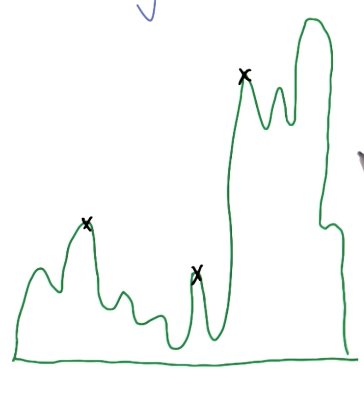
We therefore use variants such as Random Restart Hill Climbing, which performs multiple different iterations of hill climbing (which implies starting from different randomly-initialized input points). The final optimized input is calculated by comparing outputs across iterations.

Simulated Annealing#

Instead of always proceeding in the direction of ascent, other approaches may choose to select a “worse” input during search. Simulated Annealing is one such method which probabilistically selects the next input during search using temperature $T$. In this context, “annealing” references the repeated heating and cooling process applied in metallurgy.

For finite set of iterations:

• Sample new point $\mathbf{x_t}$ in neighborhood $N(\mathbf{x})$.
• Jump to this point with probability given by acceptance function $\Pr(\mathbf{x}, \mathbf{x}_t, T)$ (below).
• Decrease temperature T.

$\Pr(\mathbf{x}, \mathbf{x}_t, T) = \begin{cases} 1 & \text{if} ~f(\mathbf{x_t}) \geq f(\mathbf{x}) \\ e^{\frac{f(\mathbf{x}) - f(\mathbf{x}_t)}{T}} & \text{otherwise} \end{cases}$

Simulated annealing aims to strike a balance between exploration vs. exploitation, as opposed to the completely exploitative strategy of hill climbing.

• Exploitation: always select value which improves objective function.
• Exploration: select new values which may be associated with poorer objective function scores, with the intention of reaching a different portion of the input space (which may contain the optimal value).

Genetic Algorithms#

Finally, Genetic Algorithms refer to an alternative RO approach which combines characteristics of inputs from one iteration to generate inputs for the subsequent iteration. More specifically, genetic algorithms involve the following components:

• Population of Inputs: at each iteration, we have some group of inputs $\mathbf{X}$ which are each evaluated according to the objective function.
• Mutation: local search is performed by introducing small feature-wise mutations into inputs, and occurs according to a predefined mutation rate.
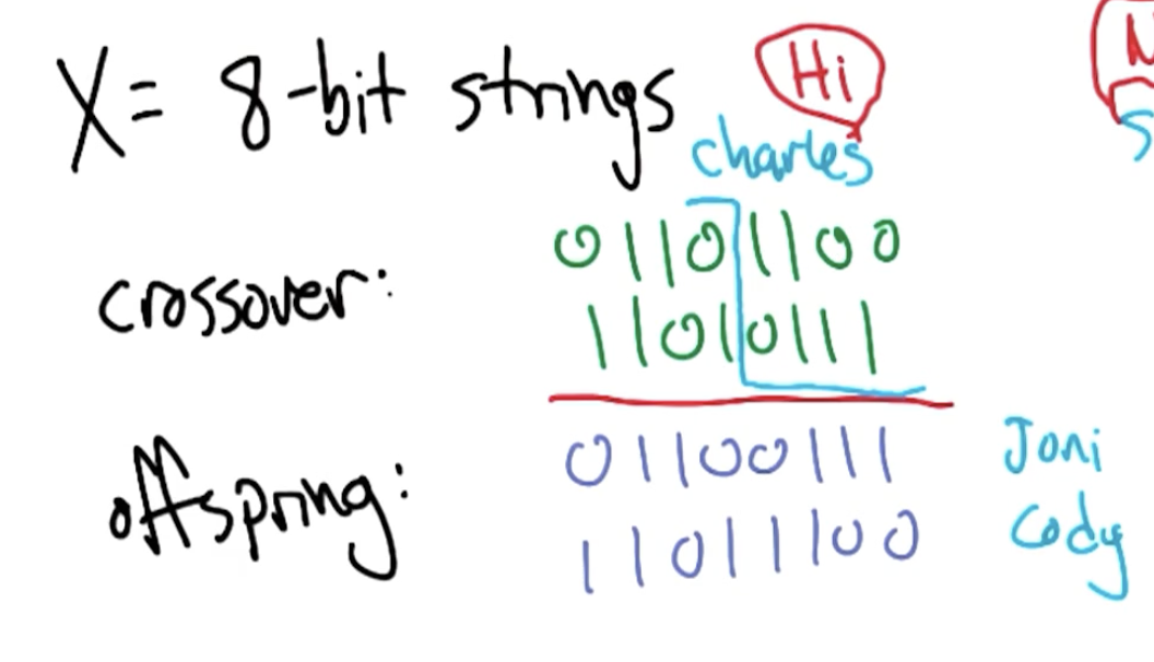
• Crossover: members of the population with better objective function scores are selected for combination.
• Generations: this process is repeated over many iterations.

Generate initial population of size $k$. Loop until convergence:

• Compute fitness for all members of population $\mathbf{x}_t \in P_t$.
• Select “most fit” individuals to be paired for crossover.
• Introduce mutation at certain rate $m_r$.

The notion of crossover assumes that different subspaces of the input are separately important for optimization. To better understand crossover, consider the following example of optimization over 8-bit strings.

MIMIC#

MIMIC is another RO method which performs optimization by directly modeling a probability distribution over inputs $\mathbf{x} \in \mathbf{X}$. More specifically, we define the following distribution:

$\Pr_{\theta}(\mathbf{x}) = \begin{cases} \frac{1}{z_\theta} & \text{if} ~ f(\mathbf{x}) \geq \theta \\ 0 & \text{otherwise} \end{cases}$

This implies that $\Pr_{\theta_{\text{max}}}(\mathbf{x})$ is a uniform distribution over optimal points, and $\Pr_{\theta_{\text{min}}}(\mathbf{x})$ is a uniform distribution over all inputs in the input space. MIMIC progresses by starting with $\theta_{\text{min}}$ and iteratively proceeding towards $\theta_{\text{max}}$.

Loop until finished:

• Generate samples from $\Pr_{\theta_t}(\mathbf{x})$.
• Set $\theta_{t+1}$ to $n$-th percentile of samples (ranked by objective function score).
• Retain only samples with $f(\mathbf{x}) > \theta_{t+1}$.
• Estimate new distribution $\Pr_{\theta_{t+1}}(\mathbf{x})$ with remaining samples.

MIMIC takes a special approach to estimating the distribution over samples via dependency trees. For more on this topic, check out the original MIMIC paper from Charles Isbell.

(all images obtained from Georgia Tech ML course materials)