Bayesian Inference

Bayesian Networks#

Probability Review#

Recall from probability theory that any Joint Distribution defines the probability distribution over multiple random variables.

$\Pr(A, B)$

The conditional distribution for two random variables defines the probability distribution for one random variable, given the other has already occurred.

$\Pr(A|B=b_1)$

X is conditionally independent of Y given Z if the probability distribution governing X is independent of the value of Y given the value of Z.

$\forall x, y, z ~~~ \Pr(X=x | Y=y, Z=z) = \Pr(X=x | Z=z)$

We can calculate the marginal distribution on a single random variable by summing (discrete) or integrating (continuous) over all possible values of the other random variables.

$\text{Discrete}: ~~~ \Pr(A) = \sum_i\Pr(A, B_i)$

$\text{Continuous}: ~~~ \Pr(A) = \int \Pr(A, B)db$

Furthermore, the chain rule of probability enables us to recover the joint distribution from a set of conditionals.

$\Pr(A, B) = \Pr(B | A) \times \Pr(A)$

What are Bayesian Networks?#

A Bayesian Network is a probabilistic graphical model representing a set of random variables and their conditional dependencies. Bayesian Networks are always directed acyclic graphs (DAGs). This enables us to perform sampling in a topological ordering such that nodes with outgoing edges are always sampled before nodes that depend on said edges.

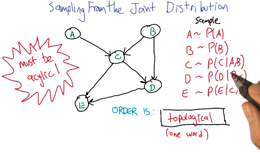
Given our Bayes Network, we can write the joint distribution as a product of conditionals, using the chain rule of probability.

$\Pr(A, B, C, D, E) = \Pr(E|C, D) \times \Pr(D | B, C) \times \Pr(C | A, B) \times \Pr(B) \times \Pr(A)$

Why is sampling useful? There are two primary cases…

• Given that we know the true joint distribution, we can 1) define the probability of observing a specific event, and 2) generate values from the distribution via simulation.
• If we do not know the true distribution, sampling allows us to perform approximate inference. Instead of doing some complex probability calculation, we can perform repeated sampling to approximate the true data-generating distribution.

Naive Bayes#

The Naive Bayes Classifier is a supervised learning approach built on Bayes Theorem. More specifically, we assume our outcome $y$ is conditionally dependent on each feature $x$, but each feature is conditionally independent of one another given the label. This point on conditional independence is known as the Naive Bayes assumption.

$\Pr(y|x_1, x_2, x_3) = \frac{\Pr(x_1|y) \times \Pr(x_2|y) \times \Pr(x_3 | y) \times \Pr(y)}{Z}$

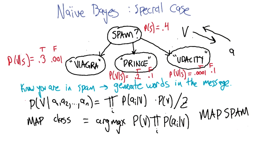
Naive Bayes is particularly useful for a number of reasons:

• inference is relatively inexpensive.
• there are relatively few parameters.
• we can directly estimate parameters with labeled data (frequencies).
• the algorithm connects inference with classification.
• it is empirically successful - the algorithm tends to do relatively well with sufficient data!

The primary drawback of the algorithm is its strong assumption. Features do not tend to be independent in the real world.

(all images obtained from Georgia Tech ML course materials)