Computational Learning Theory

What is Computational Learning Theory?#

Definition#

Computational Learning Theory (CoLT) refers to the application of formal mathematical definitions to learning systems (machinelearningmastery.com). As part of CoLT, we are interested in…

• Defining learning problems
• Demonstrating that specific algorithms work in the context of these problems
• Reasoning about how and why these problems are fundamentally difficult

CoLT is somewhat analogous to complexity analysis in computer science. For example, computing theory analyzes how algorithms use resources such as time and space. In the context of CoLT, resources such as time, space, and data are important considerations.

Inductive Learning and CoLT#

Recall that supervised learning is a form of Inductive Learning - given a set of specific instances, we would like to infer the general pattern underlying these instances.

Inductive learning involves a number of quantifiable components:

• Probability of successful training $1 - \delta$
• Number of examples to train on $m$
• Complexity of hypothesis class $H$
• Accuracy to which target concept is approximated $\epsilon$
• Manner in which training examples are presented (batch vs. online)
• Manner in which training examples are selected (more below).

With regards to the last point, how are training instances generated? We have three possible scenarios:

1. Learner asks questions of teacher to produce instances.
2. Teacher selects instances to help learner.
3. Instances are drawn from a fixed, natural distribution.

With regards to inductive learning and CoLT, we make the following definitions:

• Computational Complexity: amount of computational effort required for learner to converge.
• Sample Complexity: number of training instances necessary for learner to create successful hypothesis.
• Mistake Bounds: number of misclassifications a learner is permitted to make over an infinite run.

Computational Learning Subfields#

Version Spaces#

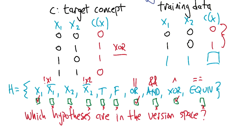
The Version Space for a machine learning problem is the set of all candidate hypotheses produced by the learning algorithm that are consistent with the true concept.

$\text{GIVEN}: ~~~ c \in H ~~~ h \in H ~~~ S \in X ~~~ c(x) \forall x \in S$

$\text{VERSION SPACE}: ~~~ VS(S) = \begin{Bmatrix} h ~~ \text{s.t.} ~ h \in H ~ \text{consistent with } S \end{Bmatrix}$

To be a member of the version space, the hypothesis should simply be consistent with the observed data. Consider the following example:

PAC Learning#

As part of any supervised learning problem, we have two main error values of interest:

• Training Error: fraction of training instances misclassified by hypothesis $h$.
• True Error: fraction of instances that would be misclassified by $h$ on a sample drawn from the true data-generating distribution $D$.

$\text{error}_D(h) = \Pr_{X \sim D} \left [ c(x) \neq h(x) \right ]$

Let us define $\epsilon$ as our error goal, and $\delta$ as our certainty goal.

$0 \leq \epsilon \leq \frac{1}{2} ~~~~~ 0 \leq \delta \leq \frac{1}{2}$

A class of concepts $C$ is considered PAC-Learnable via some learning algorithm $L$ if the learner $L$ will, with probability $1 - \delta$, output a hypothesis $h \in H$ such that $\text{error}_D(h) \leq \epsilon$ in time and samples polynomial in $\frac{1}{\epsilon}$, $\frac{1}{\delta}$, and $n$. PAC stands for probably approximately correct - more specifically, $1 - \epsilon$ correct!

A version space is considered epsilon-exhausted if all hypotheses within the version space have error lower than $\epsilon$.

$\forall h \in VS(S) ~~~ \text{error}_D \leq \epsilon$

Haussler’s Theorem bounds true error as a function of sampled training examples.

$\text{Consistent on Single Instance}: ~~~ \Pr_{X \sim D} \left[ h_i(x) = c(x) \right] \leq 1 - \epsilon$

$\text{Consistent on Sample of m Examples}: ~~~ \leq (1 - \epsilon)^{m}$

$\text{At Least One} ~ h_1, \ldots, h_k ~\text{Consistent on m Examples}: ~~~ \leq |H| \times (1 - \epsilon)^m$

Given some mathematical properties + rearrangement, we can solve for $m$ - the minimum number of training examples required to evaluate our version space - as follows:

$m \geq \frac{1}{\epsilon} \left( \ln |H| + \ln \frac{1}{\delta} \right)$

(all images obtained from Georgia Tech ML course materials)