What is Instance-Based Learning?#
Instance-Based Learning refers to a class of supervised learning algorithms which directly reference instances in the training data to generate results. As opposed to learning a model-based representation using the training data, we directly compare new instances to the training data in order to generate a prediction. This approach works well when training data is very large and diverse.
The simplest example of instance-based learning is a database lookup program. Given a set of training instances of the form , we store instances in the database with keys corresponding to and values to . Given a new instance , we compare to our set of keys to generate the prediction .
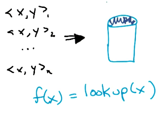
There are certain pros and cons to this approach:
- PROS:
- Not introducing any assumptions / biases via some model-based representation.
- The approach is relatively fast compared to learning for other algorithms.
- CONS:
- Models the training data exactly, which might imply overfitting.
- Generalization is nonexistent - what happens if we have a new key that isn’t currently in the database?
Instead of our simple database lookup example, we will introduce a better defined instance-based learning algorithm in the following section.
K-Nearest Neighbors#
Definition + Algorithm#
The K-Nearest Neighbors (KNN) algorithm is similar to database lookup, but relies on the notion of similarity between instances to make predictions. Given a new instance , we calculate the pairwise similarity between the new instance and each instance in our training dataset. Then, the most similar training instances inform the final prediction.
GIVEN:
- Training Data
- Query Point
- Distance Metric
- Number of Neighbors
NN =
In the case of classification, KNN predicts the mode of the most similar neighbors. For regression, KNN predicts the mean.
Hyperparameter Tuning#
As with other machine learning algorithms, KNN has a number of Hyperparameters which must be optimized specific to the task at hand:
- Distance Metric: we can choose one of many functions to represent pairwise similarity. The most common choice is Euclidean Distance, but other options such as Manhattan Distance are also reasonable.
- Number of Neighbors : the number of neighbors we use for predictions is perhaps the most important hyperparameter of the algorithm!
In order to perform hyperparameter tuning, we should use either a train-test split or cross validation to train our various hyperparameter configurations on the training partition(s), then optimize over performance on the validation (test) set.
Complexity#
Let’s compare the time and space complexity of algorithm training and inference. Assume we are given training data as a set of sorted data points with only a single feature.
| ALGORITHM | TIME COMPLEXITY | SPACE COMPLEXITY | |
|---|---|---|---|
| 1-NN | Learning | 1 | n |
| Inference | log(n) | 1 | |
| K-NN | Learning | 1 | n |
| Inference | log(n) + k | 1 | |
| Linear Regression | Learning | n | 1 |
| Inference | 1 | 1 |
Biases#
Recall that preference bias describes an algorithm’s reasoning for selecting one hypothesis over another. In the context of KNN, there are three main factors which influence preference bias:
- Locality similar points are closer in space (i.e., distance is a good representation of similarity).
- Smoothness voting / averaging over neighbors is the appropriate method for prediction.
- Equal Feature Importance distance is combined over all features in an equal fashion.
Miscellaneous Points on ML#
The Curse of Dimensionality is a problem shared across supervised learning algorithms highlighting issues associated with high-dimensional data.
As the number of features or dimensions grows, the amount of data we need to generalize accurately grows exponentially.
Consider the following example:
- We are given a training dataset containing a single integer feature with domain of and two instances: and . Our training data occupies of the input space, since there are 10 possible inputs.
- We decide to add another integer feature to the training dataset, also with domain . Our instances are now and . Now, our training data occupies of the input space - we would need 18 more different instances to cover the same portion of the input space as in the case of a single feature!
The more features we add to the problem, the more data we require to adequately represent the input space.
(all images obtained from Georgia Tech ML course materials)