Language Modeling

What is Language Modeling?#

A Language Model is a simplified approximation of language production. Language models have applications including autocomplete, summarization, translation, spelling / grammar correction, text generation, and chatbots.

The notion of fluency is particularly useful in language modeling. Fluency is a score assigned to a sequence of words that measures whether or not the words look like accurate language.

How do we Model Fluency?#

Okay, but fluency is still pretty vague here. How do we assign fluency scores to words? We can approximate fluency as a probability - what is the probability that we observe a given set of words?

$\Pr(W_1 = w_1, \ldots, W_n = w_n)$

• We have a sequence of random variables, where each word position corresponds to a distinct variable $W_i$. Each of our random variables may take on one of any value in our vocabulary $V$. $W_i \in V$
• what if we come across a word that isn’t in our vocabulary? we can add symbols to handle special cases (e.g., $<$unk$>$ for unknown, $<$sos$>$ for start of sequence, $<$eos$>$ for end of sequence).
• we may also limit our vocabulary to the top $k$ most frequently used words in a language to prevent issues with massive dimensionality.

Using the product rule of probability, we can break down our full joint distribution into a product of conditionals:

$\Pr(w_1, \ldots, w_n) = \prod_t \Pr(w_t | w_1, \ldots, w_{t-1})$

Note that all words occurring before the $t$-th word are referred to as the History of that word. One challenge here is that history grows with each word added to the sequence. We can limit history by creating a fixed lookback window.

In summary, we can approximate fluency using probability. We start with our full joint distribution over all words, then break this term down into a product of conditionals. Each $t$-th word is the word we are interested in predicting. Our goal is to approximate the conditional distribution of $w_t$ given its history using a neural network. Once we have this distribution, we can select the word which maximizes probability.

Neural Networks and Language Modeling#

Neural Language Models#

Recall that the goal of multinomial logistic regression is to produce a probability distribution over classes given a set of features.

$\Pr(Y | x_1, \ldots, x_n) \rightarrow \Pr(w_t | w_1, \ldots, w_n)$

There are certain challenges of directly applying this technique to natural language:

• with massive vocabulary, we have massive output dimensionality. solution: limit vocabulary to top $k$ words.
• we can’t use bag-of-words feature generation, since sequence is important here. solution: convert word to token - unique index in vocabulary - and use token to populate one-hot vector.

There are also certain considerations for neural network architecture. Consider a bigram language model, which uses a fixed size lookback of size 1 to predict the next word in a sequence.

$\Pr(w_t | w_{t-1})$

Even in this simple case, we have a linear mapping of $\|V\| \rightarrow \|V\|$, since our single input $w_{t-1}$ has dimensionality $\|V\|$. Extending this to a trigram language model $\Pr(w_t \| w_{t-1}, w_{t-2})$, we now have $\|V\|^2 \rightarrow \|V\|$. This is an exponential increase in the size of the input layer relative to the size of our history.

Encoders / Decoders#

One approach to reducing parameter dimensionality is to use an Encoder-Decoder neural architecture (although this isn’t the primary solution for our above problem, but rather more of an aside). Encoding and decoding can be loosely thought of as a method for compressing and de-compressing input vectors.

• Encoder: send input through compression layer (linear layer with hidden size $<$ input size) to find a more compact representation of the input. nn.Linear(|V|, 64)
• Decoder: use encodings as input to decompression layer (linear layer mapping hidden size to output dimensionality) to produce a prediction over the full range of outputs. nn.Linear(64, |V|)

The intermediate encoding is also referred to as the hidden state vector.

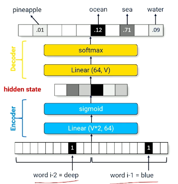
An encoder-decoder combination applied in this fashion may be thought of as an identity function. We are attempting to re-produce our original inputs using a smaller representation of our actual inputs.

Recurrent Neural Networks#

Back to our original problem - how can we apply the same neural architecture to inputs with different history sizes, and avoid the issue of exponential hidden unit dimensionality increase with increasing history? Recurrence is an architectural mechanism for processing arbitrary-length sequences. As part of recurrence, we process each time step recursively - output from the previous time step is used as input to the current time step.

How is this actually accomplished, though? As part of a Recurrent Neural Network (RNN), we use a recurrent layer as follows:

• Input: concatenation of hidden state from previous time step and current word vector.
• Output: hidden state for current time step, which is set aside for use in the next step (as well as being propagated through the rest of the network).

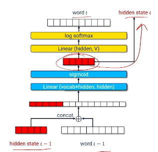
To start the training process for an RNN, we initialize our hidden state vector to zero. All subsequent time steps will use the recurrent hidden state generated from the previous time step. If we take a greedy approach to text generation, we use the previous word predicted from the RNN as the next word for input.

Generative Sampling#

How do we select our final word from the predicted log softmax distribution of scores? We take the argmax, of course. But this results in problems that might not be so obvious at first glance. In practice, our predicted distributions tend to have certain words with very high probability; this may repeat over time steps, and result in repeated words. A softer approach is to perform multinomial sampling over our predicted probability distribution to predict words in a more natural way. Even if one word dominates the predicted distribution, we won’t always select this word as our final prediction.

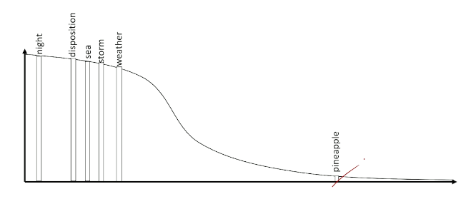
We can also apply some temperature value to scale probabilities before sampling. Assuming a temperature value $<1$, this will amplify larger scores relative to smaller scores, taking us closer to argmax behavior.

$<\frac{\log[\Pr(w_1)]}{T}, \frac{\log[\Pr(w_2)]}{T}, ..., \frac{\log[\Pr(w_{|V|})]}{T}>$

LSTMs#

Although RNNs seem like a great solution here, they have certain practical limitations:

• It is difficult for an RNN to learn a compact yet useful representation of word history.
• Subsequent time steps may “overwrite” portions of the hidden state from previous time steps.
• The hidden state may attempt to maintain all information from previous time steps, as opposed to only useful information.

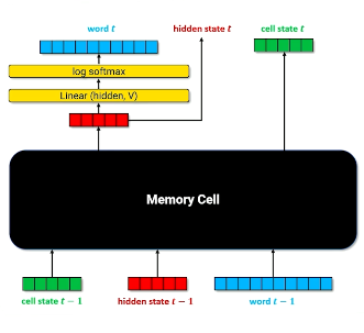
Long Short-Term Memory (LSTM) networks were created as a successor to RNNs to address their shortcomings. LSTMs use a specialized recurrent module called a memory cell to remember important parts of word history. The memory cell accomplishes by maintaining two vectors - cell state and hidden state - in combination with a structured and learnable gating mechanism:

• Forget Gate: removes irrelevant information from the previous cell state. $f = \sigma(W_{i,f}x_t + b_{i,f} + W_{h,f} h_{t-1} + b_{h,f})$
• Input Gate: adds new information to the previous cell state from the current input. $i = \sigma(W_{i,i}x_t + b_{i,i} + W_{h,i}h_{t-1} + b_{h,f}$
• Output Gate: applied to the current cell state to produce the final output of the layer. $o = \sigma(W_{i, o}x_t + b_{i,o} + W_{h, o}h_{t-1} + b_{h,o})$

Our cell state for the current time step is a function of the forget gate, input gate, and previous cell state. This is saved and used as the input cell state to the next time step. Our output for the current time step is a function of the output gate and current cell state. This produces a final hidden state, which is saved and used as the input hidden state to the next time step. The final hidden state also continues forward through the network to generate predictions for the current time step.

$c_t = (f \times c_{t-1}) + (i \times \tanh(W_{i,g} + b_{i,g} + W_{h,g} + b_{h, g}))$

$h_t = o \times \tanh(c_t)$

Note that each of the gates have elements in the range of $(0,1)$, and are multiplied element-wise by their respective terms.

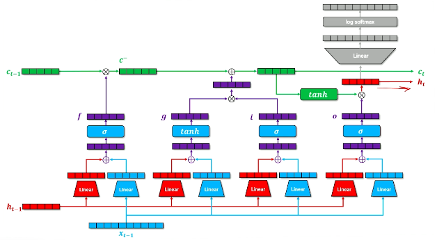
Other than the memory cell component, LSTMs follow a similar structure to an RNN.

Sequence-to-Sequence Models#

We have described language models in terms of sequential text prediction; we use a combination of current word and previous hidden state to predict the next word in the sequence. What if our task changes to generate sequences of output from sequences of input? This is especially prevalent in applications such as machine translation.

A Sequence-to-Sequence (Seq2seq) architecture is used to model sequential data, given the input and output are both sequences. Seq2seq models use separate encoder-decoder components as follows:

• Encoder is used to generate a final hidden state from the entire input sequence.
• For each term in the output sequence, we generate a prediction from the decoder. The input to the decoder is 1) the previous hidden state (starting with that from the encoder), and 2) the previous word predicted by the decoder.

Teacher Forcing refers to the training paradigm where ground truth labels are fed into the decoder for training, as opposed to using decoder predictions from previous time steps. This helps to ensure the decoder is trained on good data, and can drastically speed up / improve model results.

Attention#

Attention was introduced as part of the transformer architecture in a 2017 paper, where transformers are state-of-the-art for most modern language modeling tasks. Although we won’t get to the transformer in this module, we will establish a strong foundation by defining the attention mechanism.

Methods for recurrence involving maintaining some hidden state (whether a single vector in the case of RNNs, or two vectors in the case of LSTMs). Ultimately, this hidden state has the monumental task of encapsulating all previous (and relevant!) information within the sequence, relative to the prediction at the current time step.

Attention is an alternative approach that uses the entire set of intermediate hidden states to determine which information is relevant for the current time step. Mathematically, attention first calculates similarity between the current hidden state (query) and set of candidate hidden states (keys), then uses this similarity to calculate a weighted sum over candidate hidden states (values) to produce a final context vector.

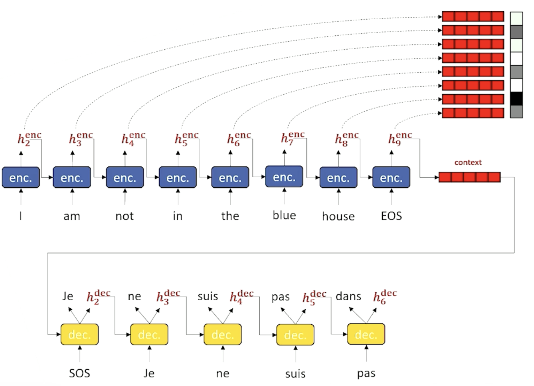
Attention offers flexibility in 1) determining which hidden states are relevant to the current step, and 2) incorporating information from many different time steps.

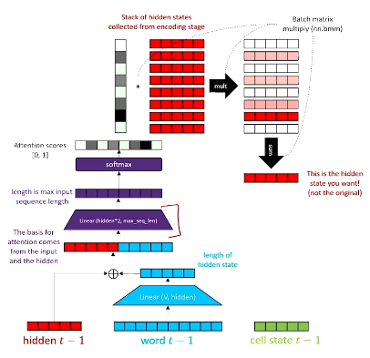
Once we have our final post-attention hidden state, we concatenate it with the original word embedding and run it through additional compression / non-linearity / decompression layers to generate our final output.

Perplexity#

While we’ve covered a bunch of neural architectures for language modeling, we haven’t touched on evaluation metrics very much. Perplexity is a common evaluation metric applied to language models to measure how confused a model is by a particular sequence of words. Mathematically, perplexity is the geometric mean of branching factor for each term in a sequence.

$\text{Perplexity}(w_1, w_2, ..., w_n) = \prod^{n}_{t=1}(\frac{1}{\Pr(w_t|w_1, w_2, ..., w_{t-1}; \theta)})^{\frac{1}{n}}$

The branching factor describes the number of things that are likely to come next; if all options are equally likely, then branching factor is equivalent to the number of options.

$\text{Branching Factor} = \frac{1}{\Pr(option)}$

$\text{Branching Factor}(w_t) = \frac{1}{\Pr(w_t|w_1, \ldots, w_{t-1}; \theta)}$

The geometric mean ensures that sequences of different length are weighted equally. Note that higher probability (confidence in our outputs) corresponds to lower perplexity; therefore, lower loss corresponds to a more confident model.

(all images obtained from Georgia Tech NLP course materials)