What is Classification?#
Classification and NLP#
Classification is a supervised learning technique in which a model is constructed to predict a discrete outcome variable. Examples of classification approaches include Naive Bayes and binary logistic regression.
Classification is particularly important in the context of natural language processing due to its many potential applications:
- spam detection: is a particular document considered spam or not?
- document topics: what topic does a particular document cover?
- sentiment analysis: are reviews positive or negative?
- text complexity: how formal / informal is a particular document? is it clear / concise?
- language / dialect detection: what language / dialect is being used in a document?
- toxicity detection: are people saying offensive things on social media?
- language generation: what word (within a finite set) should come next after a particular phrase?
The Classification Problem#
As part of any classification problem, we use some input to predict a label from a finite set of possible labels. In the context of NLP, we can frame classification as a mapping from our observed input sequence to a label .
- S: random variable representing set of all possible word sequences.
- , where represents our vocabulary (set of all possible word choices).
- represents the set of all possible output labels.
In terms of standard machine learning syntax…
- is our input variable .
- is our output variable .
Okay! So now we can move on to machine learning, right? Actually, there’s an issue with our current setup - data consisting of word sequences is relatively unstructured. How can we preprocess our data to ensure it is suitable for machine learning algorithms?
Bag of Words#
Bag of Words is one of the simplest techniques for generating a set of features from a word sequence / language document. Bag of words defines features based on word presence - for each word in our vocabulary, we create a corresponding boolean variable to indicate whether it appears in our input sequence . We can also define features for n-gram phrases as follows:
- unigram: single word.
- bigram: pair of words.
- …
Bag of words can also be applied to measure word frequency instead of presence. In either case (assuming only unigrams), we have an input feature vector , where is the dimensionality of our vocabulary. With this representation, we can now perform mathematical analyses on our input vectors to investigate patterns / trends of interest.
Classification Algorithms#
Bayesian Classification#
As a reminder, Bayesian Statistics is a branch of statistics centered around Bayes Theorem:
NLP classification is concerned with predicting the label of a document given the observed sequence of words . We can therefore apply Bayes Theorem to NLP classification as follows:
Unfortunately, some of these terms are very difficult / impossible for us to compute. The Naive Bayes Classifier helps us to avoid these computations by assuming that all features are independent. In combination with the product rule of probability, this results in the following decomposition:
$$\text{Product Rule:} ~~ \Pr(w_1, w_2, \ldots, w_d|\mathcal{L}) = \prod_i \Pr(w_i|\mathcal{L}, w_1, \ldots, w_{i-1})$$$$\text{Naive Bayes:} ~~ \Pr(w_i|w_1, \ldots, w_{i-1}) = \Pr(w_i|\mathcal{L})
$$\Pr(\mathcal{L}|w_1, w_2, \ldots, w_d) = \frac{\Pr(w_1|\mathcal{L})\Pr(w_2|\mathcal{L})\ldots\Pr(w_d|\mathcal{L})\Pr(\mathcal{L})}{\Pr(w_1)\Pr(w_2)\ldots\Pr(w_d)}$$ Okay, so now that we have our probability terms of interest, how do we calculate them? - $\Pr(w_i\|\mathcal{L})$: proportion of $w_i$ in the training data where $\mathcal{L} = \ell$. - $\Pr(\mathcal{L})$: proportion of training data with label $\mathcal{L} = \ell$. - $\Pr(w_i)$: proportion of $w_i$ across entire training dataset. Once we've applied Bayes Rule to calculate our *class probabilities* - the vector of probabilities corresponding to each of our possible labels $\ell \in \mathcal{L}$ - we can perform our final classification by taking the `argmax` of this vector. In other words, the label with the highest probability is selected as the final class assignment. Note that the `argmax` of the non-normalized class probabilities is equivalent for that to the normalized class probabilities; therefore, it is not necessary to compute the denominator term if we are not interested in recovering a valid probability distribution. #### Binary Logistic Regression **Logistic Regression** is the application of regression methodology to a discrete outcome variable. We have a set of *parameters* corresponding to each feature in our input data. Parameter values are learned via some *optimization* algorithm to produce the best set relative to some *objective function*. $$\Pr(Y=1 | X) = \sigma(\theta^Tx)$$ *Logits* are the intermediate output of logistic regression - these are the raw scores which we need to translate to class probabilities. The **Sigmoid** function is used to normalize scores from binary logistic regression to probability scale (note that sigmoid is a special generalization of softmax - we will see this later). $$\sigma(z) = \frac{1}{1 + e^{-z}}$$ 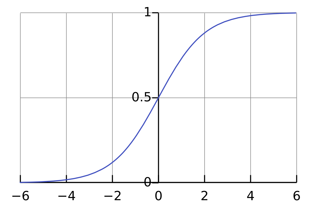 So how do we learn the optimal parameters $\theta^*$ for a logistic regression model? Simply put, the best parameter values should maximize the probability of each instance belonging to its true class label. $$\theta^* = \arg \max_{\theta \in R^d} \prod_i \Pr(Y = y_i | X = x_i; \theta)$$ That's great and all, but how can we convert this into something we can actually calculate? It turns out we can derive the following equation from our above problem statement: $$\theta^* = \arg \min_{\theta \in R^d} \Sigma_i [y_i \cdot \log[\sigma(\theta^Tx)] + (1-y_i) \cdot \log[1 - \sigma(\theta^Tx)]]$$ This is our **Loss Function**, which is the quantity we wish to minimize in the context of any supervised learning problem. More specifically, this equation represents the *binary cross entropy* between our true and estimated probability distributions over $y$. Now that we've defined a loss function that incorporates our parameters of interest ($\theta$), we can apply some optimization algorithm to identify the best set of weights. We typically use **Gradient Descent** in machine learning optimization, which iteratively updates weights by stepping in the direction of the negative gradient of the loss function w.r.t. parameters. $$\text{Gradient:} ~~\nabla L(\theta) = \begin{bmatrix} \frac{\partial{L}}{\partial{\theta_1}}, \frac{\partial{L}}{\partial{\theta_2}}, \ldots, \frac{\partial{L}}{\partial{\theta_d}} \end{bmatrix}$$ $$\text{Update Step:} ~~ \theta^{(t+1)} = \theta^{(t)} + \eta \nabla L$$ Note that as part of gradient descent, the entire training dataset is used for each step to calculate our gradient. It turns out this is very computationally demanding. Instead, we can use *Stochastic Gradient Descent (SGD)* to partition our training dataset into batches, and apply gradient descent in parallel to each batch. With this in mind, our training loop can be summarized as follows: 1. Initialize $\theta_d$ to zero or random values. 2. Iterate over *epochs* - full cycles through the entire training dataset. 1) Iterate over *batches* - smaller subsets of the training dataset; computations parallelized on the GPU. 2. Compute predictions and calculate loss. 3. Use gradient descent *update rule* to calculate new coefficients. #### Multinomial Logistic Regression **Multinomial Logistic Regression** is similar to binary logistic regression, but involves more than two categories for the outcome variable. This problem tends to be more common in NLP - for example, consider applications such as topic classification or word prediction. $$\mathcal{L} = \{\ell_1, \ell_2, \ldots, \ell_d\}; ~~\hat{y} = \{\hat{y_1}, \hat{y_2}, \ldots, \hat{y_d}\}$$ Let $k$ represent the dimensionality of our output. Instead of having a single parameter vector of dimensionality $d$, we will have a parameter matrix of dimensionality $k ~ \text{x} ~ d$. In other words, we have a set of $d$ features for each of our $k$ output classes. We still dot product this matrix with our input vector to obtain our class scores: $$z = \theta x; ~~ z \sim (k ~ \text{x} ~ 1)$$ So how can we convert these class scores to probabilities? The sigmoid function does not apply here, since we have multiple scores to pass to the function. Instead, we can use **Softmax** to calculate the probability distribution corresponding to a vector of scores. $$\text{Softmax}(z_i) = \frac{\exp(z_i)}{\Sigma_j \exp(z_j)}$$ As stated earlier, sigmoid is actually a special case of the softmax function where we assume 1) we only have two classes, and 2) the score for the negative class is 0. $$\text{Softmax}(z_0, z_1) = \begin{bmatrix} \frac{\exp(z_0)}{\exp(z_0) + \exp(z_1)}, \frac{\exp(z_1)}{\exp(z_0) + \exp(z_1)} \end{bmatrix} = \begin{bmatrix} \frac{1}{1 + \exp(z_1)}, \frac{\exp(z_1)}{1 + \exp(z_1)} \end{bmatrix}$$ $$\sigma(z_1) = \frac{\exp(z_1)}{1 + \exp(z_1)} = \frac{1}{1 + \exp(z_1)}$$ Softmax is named as such since it is basically the "soft" (differentiable) version of `argmax`. The largest score will be pushed towards 1, and everything else is shrunken towards 0. Parameter learning is very similar to binary logistic regression, but our loss function changes from binary cross entropy to *cross entropy*. Note that cross entropy is simply the generalization of entropy to $k$ output classes, whereas binary cross entropy is a special case of cross entropy. In the multi-class setting, our log loss function changes from binary cross entropy to *cross entropy*. Cross entropy includes two components: a term corresponding to the score for the correct class (which should be maximized), and a term corresponding to the scores for the incorrect classes (which should be minimized). By negating the first term, we have a minimization problem with the following function: $$ CE(y, \hat{y}) = -\Sigma_k [y_k \log(\hat{y_k})]$$ ## Computing Considerations #### Log Probabilities There are certain issues with performing calculations on computers as opposed to in their exact mathematical form: - Multiplying probabilities makes numbers very small very fast - this gives rise to *floating point precision* issues, where limited precision of the variable holding our calculation results in underflow to 0. - If any term within a product is 0, the entire product will be 0. This can happen either due to floating point precision, or when word frequencies are truly 0. To deal with the first issue, we can shift to the **Logarithmic Scale**, which converts small numbers to negative numbers. Since $\Pr(X) \in [0, 1]$, we don't have to worry about any negative inputs to the logarithmic function. 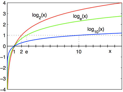 When converting to the log scale, we must update our operators accordingly. Any multiplication operations should be converted to addition. Similarly, any division operations should be converted to subtraction. $$\log(\Pr[A]\Pr[B]) \rightarrow \log(\Pr[A]) + \log(\Pr[B])$$ $$\log(\frac{\Pr[A]}{\Pr[B]}) \rightarrow \log(\Pr[A]) - \log(\Pr[B])$$ #### Smoothing But what if we have probability terms of 0 due to word absence? For example, suppose the word "cheese" is a feature, but never appears in a positive movie review. This implies $\Pr(w_{cheese}\|\mathcal{L}_+) = 0$. In practice, we modify the probability equation such that features with zero probability are never encountered - this process is known as **Smoothing**. $$\Pr_{smooth}(w_i) = \frac{1 + count(w_i)}{1 + \Sigma_{j=1}^{d} count(w_i)}$$ --- (all images obtained from Georgia Tech NLP course materials)