Modern Neural Architectures

Introduction#

Transformers are the basis of the neural architectures for some of the most successful NLP machine learning models that we have. In order to understand transformers, we build on the following structures:

• Recurrent Neural Networks (RNNs): recurrent units process time slices individually, and pass a hidden state vector between time slices to maintain information.
• Long Short-Term Memory (LSTM) networks: improve on recurrence encoding by using a memory cell to maintain both hidden and cell state across time steps.
• Sequence-to-Sequence (Seq2seq) models: use an encoder-decoder architecture to first process the input sequence (using the encoder), then iteratively construct the output sequence (using the decoder).
• Cross-Attention: neural mechanism used as part of encoder-decoder architecture which weights the importance of all intermediate encoder hidden states during an iteration of the decoder.

In this module, we will focus on how transformers combine these concepts into an efficiently elegant architecture for NLP tasks.

Transformers#

What is a Transformer?#

A Transformer is a neural architecture which has the following key components:

• Encoder / Decoder: operates on a large input window consisting of a sequence of tokens.
  • Similar to Seq2seq, the decoder takes a hidden state and entire output sequence; however, it now generates the output sequence in a single pass as opposed to token-by-token.
• Masking: hides certain input tokens to force the transformer to guess certain tokens in the sequence. Recall from Word2vec that this is a very effective method for learning meaningful word embeddings.
  • Infilling: guess word in arbitrary position.
  • Continuation: guess the word at the end of a sequence.
• Self-Attention: similar to the cross-attention mechanism, but attends to the same input sequence being processed as opposed to outputs from a previous network (e.g., encoder).

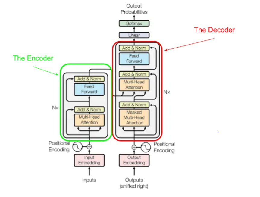
Let’s walk through each of these components in greater detail.

Transformer Encoder#

The Encoder takes an entire sequence of tokens $x_1, \ldots, x_n$ as input (for a single pass! not iterative or recurrent), then outputs a stack of hidden states with hidden size $d$ corresponding to each time slice.

$\text{ENCODER INPUT:} ~~ \begin{bmatrix} x_{(0,0)} & \ldots & x_{(0, |V|)} \\ \vdots & \ddots & \vdots \\ x_{(n, 0)} & \ldots & x_{(n, |V|)}\end{bmatrix}$

$\text{ENCODER OUTPUT:} ~~ \begin{bmatrix} h_{(0, 0)} & \ldots & h_{(0, d)} \\ \vdots & \ddots & \vdots \\ h_{(n, 0)} & \ldots & h_{(n, d)} \end{bmatrix}$

Given the input sequence of tokens and any mask indices, the encoder performs the following operations:

1. Embed the one-hots into a stack of embeddings.
   • since the encoder processes inputs in a single pass, we must include a positional embedding within our previous embedding strategy to indicate the location of each token within the input sequence.
2. Set aside a residual, which is a copy of the hidden state at a certain layer of the network. This represents a branch int he computation graph, and is especially important for combatting the issue of vanishing / exploding gradients.
3. Perform Layer Normalization to normalize all elements relative to statistics of the entire layer output, as opposed to statistics relative to each time step.
   • we can add learnable parameters to add any shifts which may be helpful to our task.
4. Apply self-attention to weight the relevance of all other time steps for each individual time step. This concept is a bit dense, so it is further explained later.
   • as part of transformer architecture, we typically use multi-headed self attention (also explained later).
5. Apply linear transformation to attention outputs. Purpose is to do whatever is necessary to ensure attention outputs are ready for the next stage.
   • “When in doubt, add in a linear layer.” - Professor Mark Riedl
6. Add back in residual component. This means each resulting embedding is a combination of the original embedding, plus some proportion of every other embedding being attended to.
7. Set aside another residual, and perform a series of 1) layer normalization, 2) expansion, 3) compression, and 4) residual addition.
8. Repeat steps 3-7 multiple times.

Note that the current encoder structure involves single-headed self-attention; each token can attend to only one other token. We can apply Multi-Headed Self-Attention to ensure that every token can incorporate many other tokens. This means that the context vector can now be related to many other tokens within the input sequence!

To implement multi-headed self-attention, we split each embedding output from the Q / K / V affine transformations within tokens into another dimension. This means that each token position can select $h$ different token positions as a separate embedding. Conceptually, this is important because each token may now be informed by the presence of many other tokens instead of only one.

Transformer Decoder#

The Decoder takes the output of the encoder (including a single final hidden state, and the set of intermediate hidden states from the attention mechanism), and generates the most probable output token per time step.

$\text{DECODER INPUT:} ~~ \begin{bmatrix} h_{(0,0)} & \ldots & h_{(0, d)} \\ \vdots & \ddots & \vdots \\ h_{(S, 0)} & \ldots & h_{(S, d)} \end{bmatrix}$

$\text{DECODER OUTPUT:} ~~ \begin{bmatrix} o_{(0,0)} & \ldots & o_{(0, |V|)} \\ \vdots & \ddots & \vdots \\ o_{(S, 0)} & \ldots & o_{(S, |V|)} \end{bmatrix}$

Given the encoder outputs and ground truth output sequence, the decoder performs the following operations:

1. Embed the one-hots into a stack of embeddings.
2. Set aside residual component.
3. Perform layer normalization.
4. Apply cross-attention such that we use the key : value pairs learned from the encoder in combination with the query being passed through the decoder.
5. Perform residual addition, layer normalization, expansion, and compression similar to the encoder.
6. Expand back to output dimensionality via the generator (output layer).

Loss is computed as KL-Divergence between each predicted token $\hat{y}_{masked}$ and its corresponding actual token $y_{masked}$.

$D_{KL} (P||Q) = \Sigma_i P(i) \log \frac{P(i)}{Q(i)}$

Self-Attention#

The Self-Attention mechanism is a bit different than cross attention, which was discussed in previous lessons. The conceptual motivation for self-attention is a hash table; we have a token at time step $t$, and we would like to identify similar (i.e., relevant) tokens at other time steps and use their hidden states in the computation for time step $t$.

More specifically, we have the following structure:

• Query: hidden state corresponding to current time step.
• Keys: set of token representations corresponding to all time steps in the sequence.
• Values: set of all hidden (feature-rich) representations corresponding to all time steps in the sequence.

We compare the query to the keys to determine similarity, then use similarity to weight values to compute some final hidden representation for the current time step. We learn each component by creating three copies of the embedding and applying separate linear transformations to each copy.

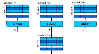
Similarity between each query vector and the full set of keys is computed via cosine similarity. Recall this is simply the dot product between each query vector and the key matrix, scaled by dimensionality.

$\text{ATTENTION WEIGHTS:} ~~ a_w = \cos(q, K) = \frac{q \cdot K^T}{|q| \times |K|}$

Once we have our similarity scores, we can convert them to a valid probability distribution (e.g., weights) using the softmax function. Finally, our hidden state is computed as a weighted sum over the value matrix.

$\text{ATTENTION RESULT:} ~~ h_a = a_w \cdot V$

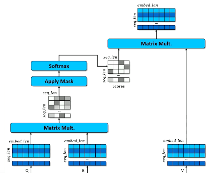
This is the process of single-headed self-attention. Multi-Headed Self-Attention is a similar mechanism in which the attention operation is applied in parallel (via some number of heads) to attend to the input in different ways.

Modern Transformers#

BERT#

The Bi-Directional Encoder Representation for Transformers (BERT) is a specific type of transformer architecture which is suited for contextual embeddings. This is a particularly useful strategy for generating word embeddings representative of semantics.

BERT uses a bi-directional self-attention structure to attend to tokens in the input sequence in both directions of the current time step (i.e., looks both ahead and behind). Note that the bi-directional nature of BERT means it is not suitable for text generation. Additionally, BERT is an encoder-only model; since we are not generating text (but rather hidden representations), we have no need to predict over the output vocabulary.

BERT is trained by randomly masking a token within an input sequence, then measuring reconstruction loss of the prediction generated by the model. This process is referred to as infilling.

GPT#

The Generate Pre-Trained Transformer (GPT) is another popular transformer architecture in natural language processing. This architecture was invented by the company OpenAI (ever heard of it??). GPT tweaks the transformer concept by masking future tokens in the sequence; this makes it suitable for text generation.

Different versions of GPT have been trained on large internet corpora over the years:

• GPT-2 (August 2019): first significant version of GPT; 774 million parameters.
• GPT-2 Large (November 2019): could be fine-tuned on specialized corpus to generate texts that look like the desired output; 1.5 billion parameters.
• GPT-3 (June 2020): cannot be fine-tuned because it lives behind an API, but is especially good at few-shot learning (i.e., doesn’t require fine tuning for most cases); 175 billion parameters.

By the time of GPT-3, the term foundation model was coined to describe a large pre-trained model trained on a diverse enough corpus to not require fine-tuning. Interestingly, prompt engineering enables GPT to pick up on a pattern in the prompt and “index into” the relevant skill portion of the transformer.

Fine-Tuning and Reinforcement Learning#

What is Fine-Tuning?#

Fine-Tuning refers to the process of pre-training a neural network on a large body of data, then continuing to train the model on a smaller specialized task. This is a form of transfer learning. Pre-trained model parameters are frozen and transferred from machine to machine. For any specific application, we may then take the frozen model and unfreeze certain portions (e.g., output layer) to specialize it to our new task.

So what’s the difference between prompting and fine-tuning? Prompting doesn’t re-train the model on a target dataset. Instead, we include information / examples in the prompt to provide the model with “clues” on how to respond.

Reinforcement Learning and Language Models#

Reinforcement Learning (RL) can also improve the quality of pre-trained language models. Recall that reinforcement learning is the field of machine learning which frames each problem as a Markov Decision Process to maximize some reward system. In the context of language models, our reward may come from human interaction via response feedback (e.g., thumbs up versus thumbs down).

Put more formally, we can apply reinforcement learning to text-based problems as follows:

1. Consider each token generated by a language model to be an action.
2. Agent generates tokens, then receives some reward. We convert reward to loss such that we have a loss minimization problem (as opposed to reward maximization).
3. The language model must decipher which token(s) were responsible for a good or bad reward. How can it pinpoint the responsible token(s)?
   • allow agent to explore different variations, and present human rater with choices.
   • train a classifier on human feedback to predict which responses are good.

(all images obtained from Georgia Tech NLP course materials)