Information Retrieval (Meta)

Introduction#

Information Retrieval (IR) refers to searching for relevant information which satisfies an informational need. More formally…

1. User submits some query corresponding to an informational need.
2. Engine calculates document relevance between query and all documents available.
3. Engine returns most relevant document to the user.

Simple IR Strategies#

Boolean Retrieval#

The simplest strategy for information retrieval is to match documents based on term similarity. In other words, how closely do the terms in the search document directly match terms within each document in the set?

The Term-Document Incidence (TDI) Matrix stores indicators for each term in our vocabulary. For each document, we have a multi-hot vector indicating which terms appear in the document.

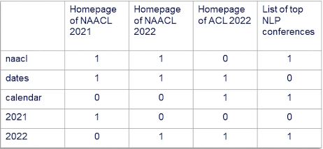
Boolean Retrieval uses the TDI matrix to identify direct matches between the query and document terms. It returns a set of unordered documents.

There are a few key issues with relying on the TDI matrix:

• The TDI is massive even for moderately-sized collections. SOLUTION: normalize terms to reduce the size of our vocabulary (e.g., stemming / lemmatization).
• The TDI is relatively sparse; any given document will contain nowhere near the number of terms in our vocabulary. SOLUTION: use an inverted index to store indices of documents in which a term appears.
• We do not capture phrases in our current definition. SOLUTION: extend the TDI to include n-grams instead of only unigram terms.

Although boolean retrieval is a good starting point, it does not typically suffice for the needs of modern information retrieval.

Ranked Retrieval#

In practice, we do care about the “order of relevance” for documents. Our result set should list more relevant documents earlier and less relevant documents later. Ranked Retrieval returns a ranked list of results sorted according to relevance.

Ranked retrieval works by calculating a relevance score for each (query, document) pair. We can substitute in whichever scoring function we are interested in using. For example, Jaccard Similarity calculates rank as the fraction of words that intersect between document $A$ and query $B$, relative to the total set of words in both document and query.

$J = \frac{|A\cap B|}{|A\cup B|}$

This scoring function has a number of issues though - for example, it assigns equal weight to words that appear commonly versus rarely, and also does not account for the frequency of query terms in the document.

A better scoring function is Term Frequency Inverse Document Frequency (TF-IDF), which is the product of term frequency and inverse document frequency.

$\text{TF-IDF}(q, d) = \Sigma_{t \in q\cap d}(1 + \log \text{TF}_{t,d}) \times \log\frac{N_D}{\text{DF}_{t,D}}$

• term frequency $TF_{t,d}$: frequency of term $t$ within document $d$.
• inverse document frequency $IDF_{t, D}$: inverse of term frequency for $t$ across all documents in set $D$, scaled by the number of documents in $D$.

TF-IDF is the best weighting heuristic in information retrieval, and is extremely power even relative to modern neural strategies.

Evaluation#

Boolean Metrics#

Assume we are given a set of unordered result documents $R = \begin{bmatrix}d_1, d_2, \ldots, d_n \end{bmatrix}$. We can use the following Boolean Evaluation Metrics to assess the quality of the results set:

• Precision: of all documents returned in $R$, what fraction are relevant? (positive predictive value)
• Recall: of all documents which are relevant in the entire collection, what fraction appear in $R$?

Ranked Metrics#

Now assume we have our set of result documents, but they are ranked as opposed to unordered. We can define the following Rank-Based Evaluation Metrics:

• Precision at k (Pr@k): precision of documents within the top-k retrieved results.
• Mean Average Precision (MAP): mean of average precision over all queries in consideration.
  • Average Precision: average of Pr@k, where $k$ is set to the true document rank.
• Mean Reciprocal Rank (MRR): defines $k$ as the rank of the first retrieved relevant document, then takes the mean of $\frac{1}{k}$ across queries. Appropriate in cases where only a single relevant document is enough.
• Normalized Discounted Cumulative Gain (NDCG): only metric which accounts for non-binary relevance.
  • Given a list of documents sorted according to relevance rating, we can calculate cumulative gain as $r_1 + r_2 + r_3 + \ldots + r_n$
  • Discounted cumulative gain gives more weight to higher ranked documents $r_1 + \frac{r_2}{\log(2)} + \frac{r_3}{\log{(3)}} + \ldots + \frac{r_n}{\log{(n)}} = r_1 + \Sigma_i \frac{r_i}{\log(i)}$
  • Finally, normalized DCG scales by the maximal DCG value at rank $n$ to account for queries with varying number of relevant results (i.e. different values of n).

Evaluation of IR algorithms is typically accomplished using a benchmark dataset, which should have the following components for any IR task: collection of documents, set of queries, and relevance labels for each (query, document) pair.

Probabilistic IR#

Binary Independence Model#

Instead of assigning relevance to (query, document) pairs in a hard-coded fashion - whether binary in the case of boolean retrieval or continuous in the case of ranked retrieval - we can use a probabilistic approach to model the probability of relevance $\Pr(R = 1 \| q, d)$. This probability can then be used to rank documents for return.

The simplest probabilistic information retrieval model is the Binary Independence Model (BIM), which represents queries and documents as binary term incidence vectors.

$\text{QUERY:} ~~ \begin{bmatrix} d_1, \ldots, d_{|V|} \end{bmatrix}$

$\text{DOCUMENT:} ~~ \begin{bmatrix} q_1, \ldots, q_{|V|} \end{bmatrix}$

Our ranking score function is the odds that the document is relevant versus not relevant.

$\text{BIM SCORE:} ~~ \frac{\Pr(R=1|d, q)}{\Pr(R=0|d, q)} = \frac{\Pr(d|R=1, q)}{\Pr(d|R=0, q)}\frac{\Pr(R=1|q)}{\Pr(R=0|q)}$

• $\frac{\Pr(R=1\|q)}{\Pr(R=0\|q)}$ measures the odds of query relevance; given a fixed query, this is constant.
• As part of the binary independence model, we assume that each variable is independent. This enables us to calculate probability as a product over terms in our vocabulary.

$\frac{\Pr{(d\|R=1, q)}}{\Pr{(d\|R=0, q)}} = \prod_{d_i = 1}\frac{p_i}{r_i} \prod_{d_i = 0}\frac{1-p_i}{1-r_i}$

$p_i = \Pr(d_i=1 | R = 1, q)$

$r_i = \Pr(d_i = 1|R=0, q)$

The final ranking score is calculated as follows, where probabilities are derived via a training dataset.

$\Sigma_{x_i=d_i=1} \log \frac{p_i(1-r_i)}{r_i(1-p_i)}$

BIM has a number of assumptions that are often not accurate in practice:

• terms are not independent
• terms not present in the query do not impact ranking
• the representation of query / document as boolean is not great

So what else can we do?

Best Match 25#

Best Match 25 (BM25) is another probabilistic information retrieval method that alters TF-IDF to incorporate document length $L$.

BM25 calculates document score as follows:

$\Sigma_{i\in q} \log \frac{N}{\text{DF}_i} \frac{(k+1)\text{TF}_i}{k((1-b) + b \frac{L}{\text{avg}(L)}) + \text{TF}_i}$

This model has only two free parameters:

• $k$: controls term frequency weight.
• $b$: controls document length normalization.

Neural Information Retrieval#

Machine Learning and IR#

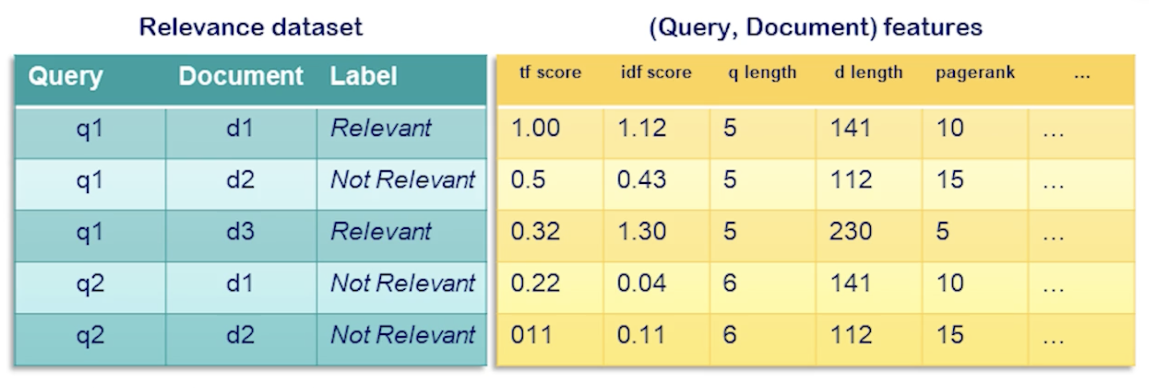
Information retrieval can be framed as a supervised learning problem where we attempt to learn the function mapping a query : document pair to a relevance score. Relevance score may be binary (binary classification), multi-class (multinomial classification), or continuous (regression).

$f(q,d) \rightarrow s$

Training occurs as it would for any other supervised ML problem. We have a training dataset with (query, document) pairs identifying each row, an outcome variable of interest, and features pertaining to each (query, document) pair. For example, here’s a sample dataset for IR binary classification:

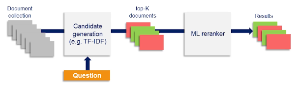
However, we now have the problem where we must perform inference for each (query, document) pair. This is very computationally expensive, especially compared to the fast classical IR methods. One solution is to first run classical retrieval for a query, then run the machine learning model on the shorter list of the top $k$ results from classical retrieval.

Framing IR as a binary classification problem is helpful, but not perfect. Ranking is more useful since we can determine whether a document is more or less relevant than competing documents. We can apply Pair Ranking to address this limitation.

• Instead of modeling the single relevance of a document in isolation, we model the outcome that a given document is more relevant than another. $\Pr(R=1\|d_i, q) \rightarrow \Pr(r_{d_i} > r_{d_j} | q)$
• The model still outputs some score for each document, but we transform this score using the sigmoid of the differences in score, as opposed to the sigmoid of the score itself. $\sigma(s_i - s_j)$
• This implies we change our loss function from simple cross entropy, to cross entropy with the predicted score being $\sigma(s_i - s_j)$.

Embedding-Based Retrieval#

Recall that we can represent both queries and documents as multi-hot vectors of dimensionality $\|V\|$. Since we have vector representations, we can calculate similarity using something like Cosine Similarity.

$\frac{q \cdot d}{|q| \times |d|}$

Unfortunately, multi-hot vectors don’t do a great job of capturing word semantics. We can instead use Embeddings to represent our queries and documents, since they tend to do a better job of representing word context / meaning.

We can substitute the embedding method as desired; for example, Word2vec can be used to generate vector representations for each word in our vocabulary. Given a set of word embeddings, we can compute an embedding at the query / document level as follows:

$Q = \frac{1}{L_q} \Sigma_i w_i$

$D = \frac{1}{L_d} \Sigma_i w_i$

Note that these embeddings correspond to the mean word embedding for each document. Once we have a single embedding per document / query, we can compute distance between the two vectors using something like cosine similarity. However, we have a problem - similar to the case of binary classification, inference on each (query, document) pair is infeasible. We can be more efficient by first clustering documents (e.g., k-nearest neighbors), then performing two-stage retrieval as follows:

1. Retrieve $k$ closest clusters to query.
2. Perform brute-force search over documents in retrieved clusters.

Alternative methods such as Dual-Embedding Space Model (DESM) use normalized embeddings with different embeddings for query and document ($IN$ vs. $OUT$). As part of DESM, we calculate the mean of cosine similarity for each word embedding, as opposed to the cosine similarity of the mean word embedding per document.

$\text{DESM}(d,q,w) = \frac{1}{N_q} \Sigma_i \bar{D}^T_{OUT} \bar{w}_{IN, i}$

Yet neither of these approaches beat classical methods such as BM25. Researchers have found that BERT embeddings can be altered to better suit the task of IR (since vanilla BERT embeddings were not very successful).

(all images obtained from Georgia Tech NLP course materials)