Denoising Diffusion Probabilistic Models

Introduction#

(notes for this intro section obtained from IBM: What are Diffusion Models?)

Diffusion Models are a class of generative models, which broadly seek to estimate the joint probability distribution of our data $\Pr(X)$ in order to sample new (synthetic) instances. Diffusion models are most commonly applied to image generation and other computer vision tasks.

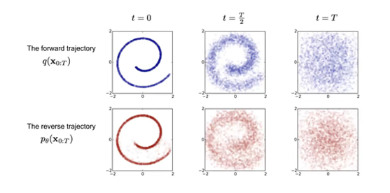
The primary idea behind diffusion modeling is that we will progressively “diffuse” samples with random noise, eventually destroying the original input instance. The diffusion model learns to perform denoising to probabilistically reconstruct the original instance. A trained diffusion model takes in random noise as input, and produces an instance of the target class.

Denoising Diffusion Probabilistic Models (DDPMs) were introduced in 2020 as competitors to state-of-the-art image generation methods such as Generative Adversarial Networks (GANs). As of today, DDPMs are the most dominant family of models for image generation.

DDPMs#

Overview of Modeling Process#

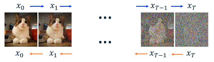
DDPM process image data in two main steps:

1. Forward Diffusion: iteratively add noise to an input image, eventually producing an image of simply noise. Noise is typically assumed to be Gaussian $\mathcal{N}(0, I)$.
   • Diffusion is repeated over many time steps $T$, with intermediate representations of the image $x_t$ produced at each step.
   • $x_0$ is always the input image, and $x_T$ is always the pure noise version of the image.
   • NOT a neural network. Instead, we are simply adding Gaussian noise to the input.
2. Denoising: generate an image from noise by iteratively removing noise from the final noised image $x_T$.
   • Implemented as a neural network.

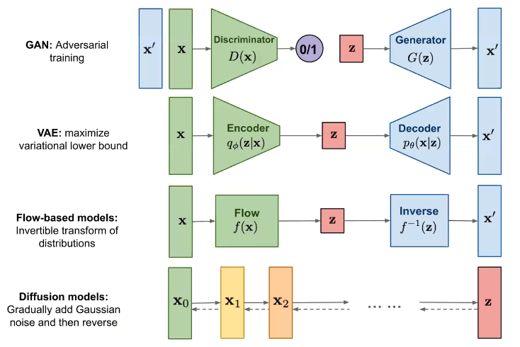
Compared to other generative models, diffusion models are relatively unique in their methods for generation.

Whereas the forward diffusion process is well-defined, the denoising diffusion process is the learned part of DDPMs. Let’s step through the math of each step more formally.

Step 1: Forward Diffusion#

As previously mentioned, the forward process of a diffusion model iteratively adds noise to the original input image $x_0$ to produce some final image of only noise $x_T$. Forward diffusion is sometimes referred to as encoding, even though we don’t use a neural network to transform the input.

We can represent the forward diffusion process as a Markov Chain - a stochastic process describing a sequence of possible events, in which the probability of the current event only depends on the previous event (Markov Property). Note that a Markov Chain is a special case of the Chain Rule of Probability, which states that we can decompose a joint probability distribution into a product over all conditionals.

$\text{CHAIN RULE}: ~~~ \Pr(e_1, e_2, e_3) = \Pr(e_3 ~ | ~ e_2, e_1) \times \Pr(e_2 ~ | ~ e_1) \times \Pr(e_1)$

$\text{MARKOV CHAIN}: ~~~ \Pr(e_1, e_2, e_3) = \Pr(e_3 ~ | ~ e_2) \times \Pr(e_2 ~ | ~ e_1) \times \Pr(e_1)$

Applied to the forward diffusion process, we have…

$q(x_{1:T} ~ | ~ x_0) = \prod_{t=1}^T \Pr(x_t ~ | ~ x_{t-1})$

… where each conditional distribution is estimated by a conditional Gaussian as follows:

$q(x_t ~ | ~ x_{t-1}) = \mathcal{N}(x_t; (\sqrt{1-\beta_t})x_{t-1}, \beta_tI)$

• $\mathcal{N}(x_t)$ indicates we are defining the Gaussian for time step $t$; $x_t$ is not actually part of the parameter definition here.
• Note that the parameters of our Gaussian is changing as a function of time step. More specifically, the variance schedule $\beta_t$ increases with time such that $\beta_t > \beta_{t-1}$, and is used to control the parameters of our Gaussian distribution.
  • Mean $(\sqrt{1-\beta_t})x_{t-1}$: at each time step, scale down the previous image $x_{t-1}$ by a small amount. Note that $\sqrt{1 - \beta_t}$ will decrease as time step increases. Conceptually, this represents the signal preservation portion of our distribution.
  • Covariance $\beta_t I$: at each time step, define covariance as a function of $\beta_t$. Note that $\beta_t$ will increase with time, meaning covariance will also increase. Conceptually, this represents the noise addition portion of our distribution (i.e., more variance = more noise).

We can actually unroll our computations over time to produce a distribution of any intermediate output $x_t$ conditioned on the original input $x_0$.

$q(x_t ~ | ~ x_0) = \mathcal{N}(x_t; \sqrt{\bar{\alpha}}_t x_0, (1 - \bar{\alpha}_t)I)$

$\alpha_t = (1 - \beta_t), ~~~ \bar{\alpha}_t = \prod_{s=1}^t \alpha_s$

Recall in the case of VAEs, we introduced the Reparameterization Trick to avoid sampling directly within our computation graph (which would prevent backpropagation, since sampling is a non-differentiable operation). We apply the same trick in the case of DDPMs.

$x_t = \sqrt{\bar{\alpha}_t}x_0 + \sqrt{1 - \bar{\alpha}_t} \epsilon, ~~~ \epsilon \sim \mathcal{N}(0, 1)$

Step 2: Denoising Diffusion#

During the reverse process, we denoise our completely-noised instance $x_t$ to generate an instance of the original type. Whereas the forward diffusion step is well-defined, the reverse diffusion step is completely learned by our neural network. Denoising as part of DDPMs is sometimes referred to as the decoding portion of the full process.

Similar to the case of forward diffusion, the denoising process can be thought of as a Markov Chain of conditional Gaussians.

$p_{\theta}(x_{0:T}) = \Pr(x_T) \times \prod_{t=1}^{T} p_{\theta}(x_{t-1} ~ | ~ x_t)$

$p_{\theta}(x_{t-1} ~ | ~ x_t) = \mathcal{N}(x_{t-1}; \mu_{\theta}(x_t, t), \Sigma_q(t))$

Note that while the Markov Chain looks familiar, the estimate of each conditional Gaussian distribution has changed. Our distribution parameters are estimated via a neural network. For simplicity, we typically only estimate the mean vector $\mu_{\theta}$ and define covariance as the corresponding covariance from the forward diffusion process $\Sigma_q(t)$.

How does our neural network estimate the conditional distribution at each time step? The high-level intuition is to derive some ground truth denoising distribution $q(x_{t-1} ~ \| ~ x_t, x_0)$, then train a neural network to generate an estimate of this distribution $p_{\theta}(x_{t-1} ~ \| ~ x_t)$. As such, our Loss Function for optimization can be formulated as the KL Divergence between our ground truth and estimated probability distributions.

$\arg \min_{\theta} \text{D}_{KL} ~~ q(x_{t-1} ~ | ~ x_t, x_0) ~ || ~ p_{\theta}(x_{t-1} ~ | ~ x_t)$

Since we know the noise added at each time step - each conditional distribution of the forward diffusion process was created via our $\beta_t$ specification - we can directly calculate our ground truth distributions.

$q(x_{t-1} ~ | ~ x_t, x_0) = \mathcal{N}(x_{t-1}; \mu_q(t), \Sigma_q(t))$

$\mu_q(t) = \frac{1}{\sqrt{\alpha_t}}(x_t - \frac{\beta_t}{\sqrt{1 - \bar{\alpha}_t)}}\epsilon), ~~~ \epsilon \sim \mathcal{N}(0, I)$

Therefore, assuming identical variance $\Sigma_q(t)$, we can decompose our loss function from KL Divergence between predicted and ground truth denoising conditional distributions, to simple mean squared error between the actual noise added and our network’s prediction of noise added. (this involves a ton of math, so I will not consider the derivation here). This implies we must store the noise added during forward diffusion for use in the final loss function.

$\arg \min_{\theta} \text{D}_{KL} = \arg \min_{\theta} || \epsilon - \epsilon_{\theta}(x_t, t) || ^2$

This implies we design our neural network to predict noise $\epsilon_{\theta}$ as opposed to the parameters of the noise distribution.

“Anytime you can make the neural network estimate something smaller or simpler, compared to something that’s more complicated, you should choose the simpler option.”

• Zsolt Kira

Practical Considerations#

During Model Training, we perform forward diffusion by iteratively adding noise to our input image. Once we have a noisy image, we feed it to our decoder neural network to estimate noise $\epsilon_{\theta}$.

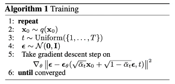
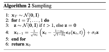
For Model Inference, we provide the neural network with a noised image $x_T$, and iteratively feed $x_t$ to the denoiser process to generate $x_{t-1}$ until reaching $x_0$.

As a final summary of the diffusion process, consider the following illustration. Forward diffusion progressively noises the original input image until reaching a point of compete noise. Conversely, reverse diffusion progressively denoises the final noised image to reproduce a valid input.