Generative Modeling

Introduction#

To this point, we’ve only considered supervised applications of deep learning. Yet there are many real-word scenarios where supervised learning is not practical. In this section, we will explore such scenario one such scenario - generative modeling - and see how deep learning frameworks can be altered to fit problems of this class.

Types of Machine Learning#

Recall that Machine Learning consists of three major subfields:

• Supervised Learning: function approximation. Given input $X$ and labels $y$, we are interested in learning the functional mapping from $X$ to $y$.
  • Learning Output: $f : X \rightarrow y, ~~ \Pr(y ~ \| ~ X)$
  • Examples: regression, classification
• Unsupervised Learning: data description. Given data $X$, we are interested in learning more about the structures present in the data.
  • Learning Output: $\Pr(X)$
  • Examples: clustering, density estimation
• Reinforcement Learning: reward maximization. Given some action-taking agent and a reward framework, we are interested in teaching the agent to select actions to maximize reward.
  • Learning Output: decision-making policy to select an action $a$ given state $s$; $\pi(s, a)$

Deep Learning is a collection of methods involving compositions of differentiable functions which can be applied across each of these fields. The defining characteristic of deep learning relative to classical (i.e., non-DL) machine learning algorithms is that feature extraction is bundled into the learning algorithm as part of end-to-end learning.

Deviations from Supervised Learning#

So what are some example scenarios where traditional supervised learning is not sufficient?

• Few-Shot Learning: learning (model training) is conducted on a base dataset with many labels. At inference time, we provide the model a support set consisting of labels the model has never seen before (with 1-5 instances per label). The support set may be provided as part of a prompt-based model (in-context learning) or in a transfer learning setting (fine-tuning).
• Semi-Supervised Learning: data consists of relatively few labeled instances, and many unlabeled instances. Train model on labeled part of data, then use model to generate labels for the unlabeled instances (only in cases where the model is very confident). Then, use newly-labeled data to re-train the model and repeat the process.
• Autoencoders: given a dataset $X$ with no labels (unsupervised learning), train an encoder-decoder structure to produce some low-dimensional embedding as part of dimensionality reduction. Objective is to minimize the difference between encoder inputs and decoder outputs.
• Generative Models: estimate the joint probability distribution over input features in order to sample from (i.e., generate) this estimated distribution.

In this module, we will take the same building blocks of deep learning covered in previous lessons and apply them to a range of new scenarios. Modifications will be made to overall neural architecture, loss functions, and training procedures as appropriate for the task at hand.

Generative Models: An Overview#

Generative Models estimate the joint probability distribution over input features $\Pr(X)$, which can then be sampled from to create synthetic instances.

Note that the general problem of density estimation has existed prior to the popularization of deep learning. Classical unsupervised learning techniques such as Gaussian mixture modeling are commonly used in this domain, but tend to fail in high-dimensionality settings. From a modern perspective, neural density estimation methods are much more powerful, especially in terms of synthetic data generation.

Whereas discriminative models model the conditional distribution $\Pr(y ~ \| x)$ to discriminate between class labels (i.e., perform classification), generative models focus on estimating the distribution over input features $\Pr(X)$. This is a very complex distribution - how can we go about modeling it? Similar to discriminative models, we can use a parametric model to assume some structure for our distribution, then estimate the best set of parameters using maximum likelihood theory.

$\theta^* = \arg \max_{\theta} \prod^m_{i=1} \Pr_{\text{model}}(x^{(i)}; \theta)$

Since the problem is so difficult, a wide range of methods have been developed for generative modeling.

Types of Generative Models#

PixelRNN and PixelCNN#

The first set of generative models we will consider represent the joint distribution $\Pr(X)$ as an explicit, tractable density. We use the chain rule of probability to decompose our joint distribution into a product of conditional distributions. This is very similar to the approach used for word sequence probability in language modeling.

$\Pr(X) = \prod_{i=1}^p\Pr(x_i ~ | ~ x_1, \ldots, x_{i-1})$

However, we already have a problem - this type of model seems to imply some form of ordering across our features $x_i$. Ordering is inherent to the problem at hand and may require certain assumptions. For the remainder of this section, consider the case where our input data consists of 2D images.

Pixel RNN uses a recurrent neural network (RNN) to model the joint probability distribution over input pixels. Here, order is assumed to start at the top left pixel and spread southeast in an equal fashion.

$\Pr(X_{\text{image}} = \prod_{i=1}^{H \times W} \Pr(x_i | x_1, \ldots, x_{i-1})$

From here, we can train our Pixel RNN similar to any other RNN (recall the language model section and concepts such as teacher forcing). There are certain cons to this method, including the slow sequential nature of autoregressive generation and relatively limited neighborhood context for each pixel.

Pixel CNN is an alternative approach which uses a convolutional neural network (CNN) to model the joint probability distribution over input pixels. As part of this method, we represent the conditional distribution as a convolution layer. This results in a larger context - i.e., receptive field - but comes with practical considerations such as masking out “future” pixels which have not yet been generated.

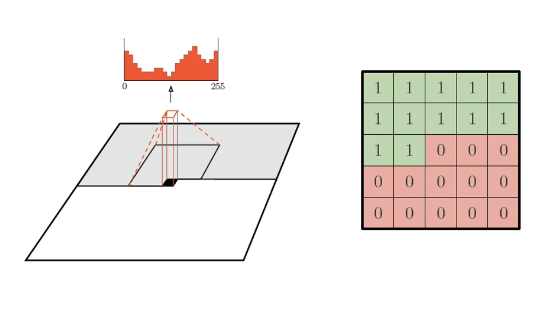
Pixel CNN results in faster model training compared to Pixel RNN, but it is still a relatively slow process since we iteratively generate for each pixel. Both methods are interesting in terms of 1) generating the remainder of occluded images, and 2) generating images from scratch.

GANs#

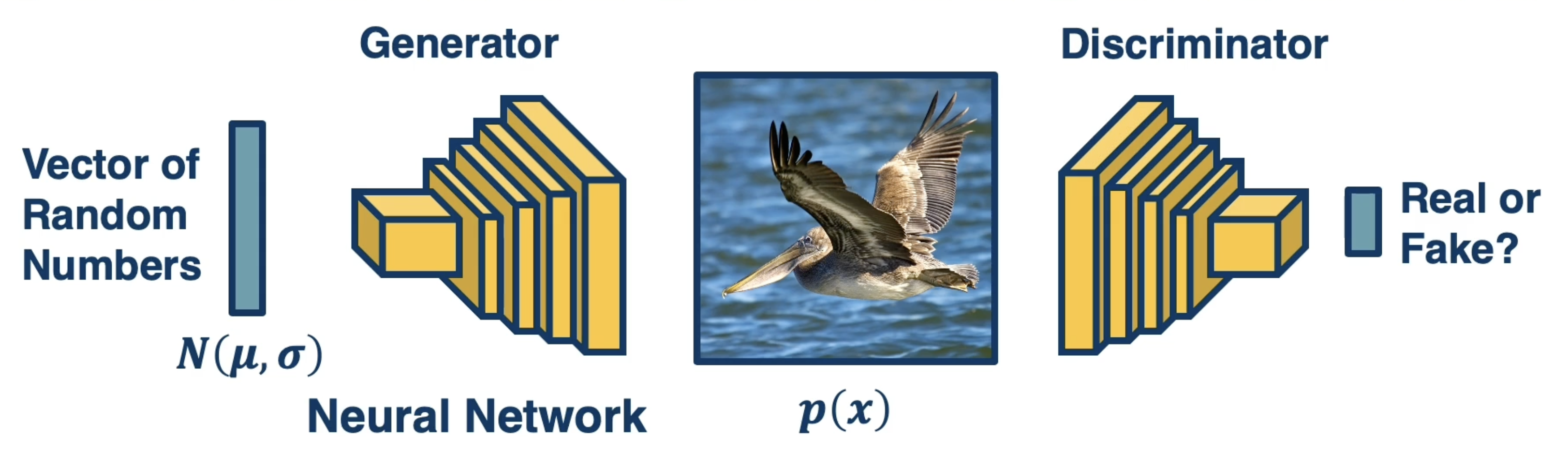
Generative Adversarial Networks (GANs) do not explicitly learn the joint probability distribution $\Pr(X)$, but instead implicitly model density by learning to generate samples from $\Pr(X)$. How is that even possible?

GANs use two networks to train in an adversarial (oppositional) fashion:

• Generator: takes an input of random values and generates a synthetic instance.
  • random values are required as input since the generator itself is fully deterministic.
  • conceptually, the generator is approximating sampling from the true joint distribution.
  • GOAL: update weights to improve realism of generated images.
• Discriminator: takes a synthetic instance as input and classifies as real or fake.
  • works in opposition to generator; if the generator is doing a poor job of creating synthetic instances, the discriminator will be able to distinguish real vs. fake much more easily.
  • fed a combination of real and synthetic instances at each iteration.
  • GOAL: update weights to better discriminate between real and fake.

Since we are really performing two optimizations simultaneously. This translates to a composite optimization problem incorporating components for each network.

$\min_G \max_D V(D, G) = \mathbb{E}_{x \sim \Pr_{data}(x)} [\log D(x)] + \mathbb{E}_{z \sim \Pr_z(z)}[\log(1 - D(G(z)))]$

• The second expectation represents the performance of the discriminator on synthetic data.
  • $z$ is our noise vector - a collection of random values fed as input to the generator.
  • $G(z)$ estimates sampling from the joint probability distribution to generate a new instance.
  • $D(G(z))$ is the discriminator’s estimate for probability that the synthetic instance is real (binary classifier with {0: fake, 1: real}.
• The first expectation represents the performance of the discriminator on real data.
  • $x$ is a real instance obtained from the real joint distribution (i.e., training data).
  • $D(x)$ is the discriminator’s estimate for probability that the real image is real.

The weights of the generator are optimized to minimize this function $\min_G$, whereas the weights of the discriminator are optimized to maximize this function $\max_D$.

• Generator Loss (minimize): $\frac{1}{m} \Sigma_{i=1}^m \log (1 - D(G(z^{(i)})))$
• Discriminator Loss (maximize): $\frac{1}{m} \Sigma_{i=1}^m \log(D(x^{(i)}) + \log(1 - D(G(z^{(i)})))$

As part of optimization, we apply stochastic gradient descent (SGD) by alternating optimization between the generator and discriminator. Performance tends to be better when the discriminator is allowed to train for $k$ iterations between generator training iterations.

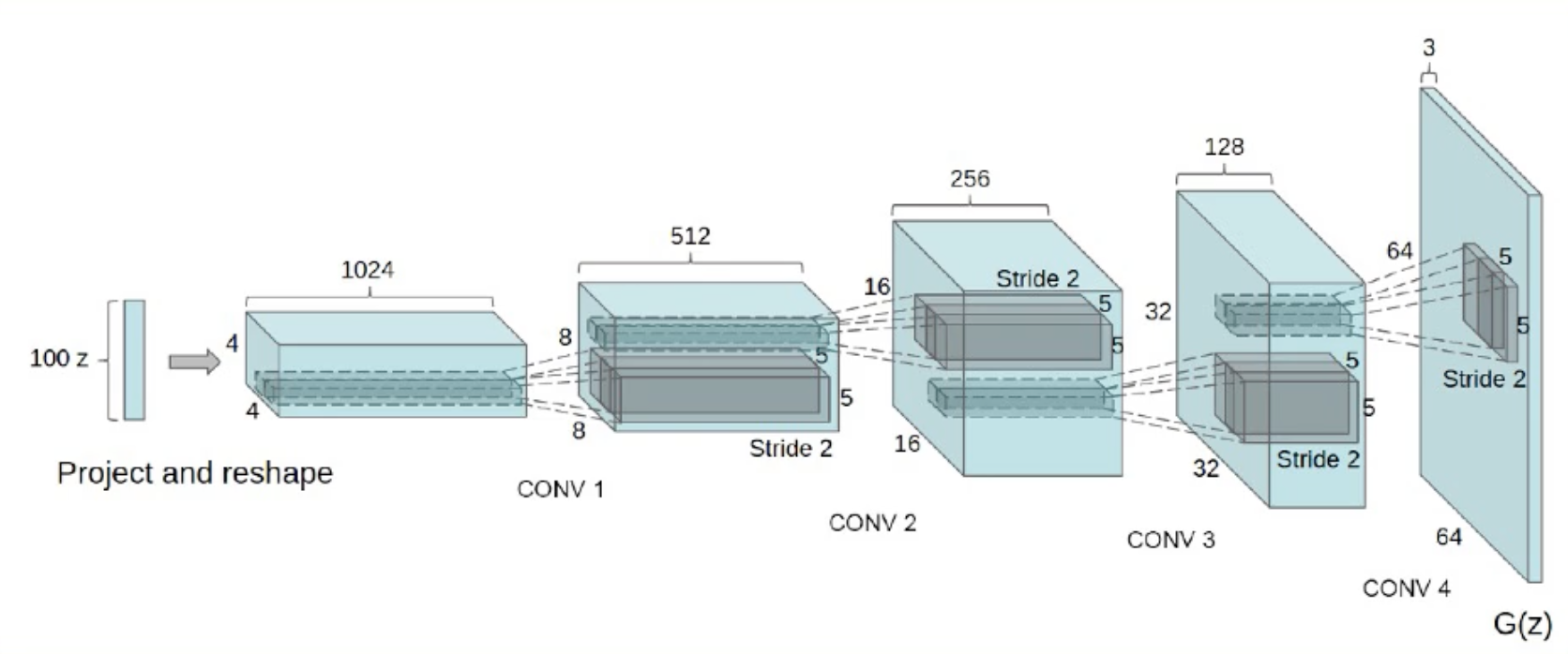
Different neural architectures are more stable for training GANs - Deep Convolutional GANs are a very common implementation.

VAEs#

(refer to CMU Variational Autoencoders Lecture for supplemental information)

$\underline{\text{CONCEPTUAL OVERVIEW}}$

Variational Autoencoders (VAEs) are another type of generative model which explicitly model the joint probability distribution $\Pr(X)$ via approximation. Recall that autoencoders generate some low-dimensional embedding as part of an encoder-decoder architecture - their primary purpose is to perform dimensionality reduction to a meaningful feature representation.

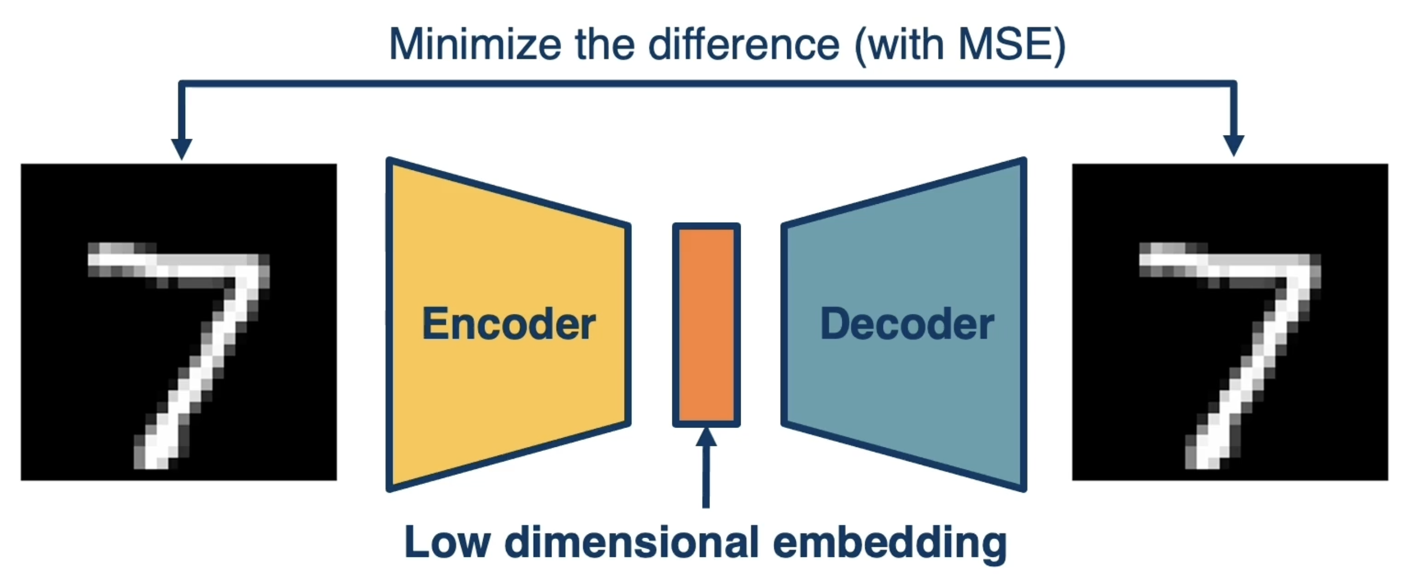
The low-dimensional embedding represents some combination of hidden / latent variables $Z$. The primary purpose of a traditional autoencoder is to generate an encoder-decoder pairing such that reconstruction error is minimized; in other words, autoencoders are concerned with directly reproducing the input using some meaningful latent representation.

VAEs have a slightly different goal. While we are still interested in generating some informative latent representation, we don’t want to reproduce the input. Rather, our system should generate new instances of the input in a stochastic fashion. VAEs are therefore framed to estimate distribution parameters as opposed to data itself. For example…

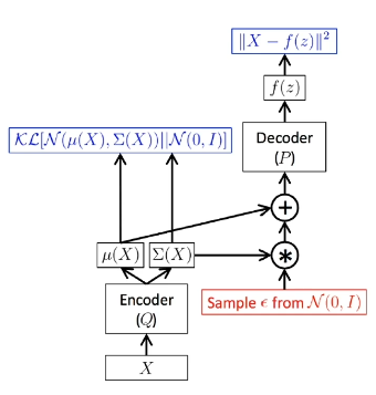
• Encoder: recognition model. Learns the mapping from input $X$ to latent-generating distribution $\Pr(Z ~ \| ~ X)$ by estimating its parameters.
  • does NOT generate a latent vector $Z$, but rather the distributional components required to sample from $\Pr(Z ~ \| ~ X)$ to generate a new instance of $Z$.
  • in the case of a Gaussian VAE (most common), our output is a vector of means $\mu_Z$ and covariance matrix $\Sigma_Z$ defining the multivariate Gaussian distribution over latent features.
• Decoder: generative model. Learns the mapping from latent representation $Z$ to data-generating distribution $\Pr(X ~ \| ~ Z)$ by estimating its parameters.
  • $Z$ is sampled from encoder output prior to feeding to decoder as input.

Okay, this is all still a little too abstract. Let’s dive into the mathematical details.

$\underline{\text{DERIVATION OF LOWER BOUND}}$

Recall that our optimization problem in the case of generative modeling is to find model parameters $\theta$ to maximize likelihood. With a bit of hand-waving, we typically write likelihood as $\Pr(X)$, meaning we are interested in maximizing the probability of observing our data $X$.

$\text{VAE OPTIMIZATION PROBLEM}: ~~~ \arg \max_{\theta} \Pr_{\theta}(X)$

Given the Law of Total Probability, we can reformulate $\Pr(X)$ by marginalizing over some latent representation $Z$. Note that the specification of $Z$ (e.g., dimensionality) is arbitrary; the same logic applies for any $Z$ specified by the VAE designer.

$\Pr(X) = \int \Pr(X ~ | ~ Z; \theta) \Pr(Z) dZ$

Great! So we have a formula to directly calculate $\Pr(X)$, which is the term we’re interested in maximizing. So we’re done!! Wishful thinking. The integral over $Z$ is intractable due to 1) the high dimensionality of $Z$, and 2) there being no closed form solution. So it turns out we can’t really use this definition here.

Instead, VAEs use some pretty cool math to approximate $\Pr(X)$ as follows:

1. Start with $\log \Pr(X)$. We can set this equal to an expectation over the latent distribution defined by the encoder.
   $\log \Pr_\theta(X) = \mathbb{E}_{z \sim q_\phi(Z | X)} [\log \Pr_{\theta}(X)]$

2. Apply Bayes Rule to redefine the expectation.
   $\log \Pr_{\theta}(X) = \mathbb{E}_Z [\log \frac{\Pr_{\theta}(X | Z)\Pr_{\theta}(Z)}{\Pr_{\theta}(Z | X)}]$
   $\Pr(Z|X) = \frac{\Pr(X | Z)\Pr(Z)}{\Pr(X)} \rightarrow \Pr(X) = \frac{\Pr(X | Z)\Pr(Z)}{\Pr(Z | X)}$

3. Perform algebraic trick by multiplying fraction by term involving encoder distribution.
   $\log \Pr_{\theta}(X) = \mathbb{E}_Z [\log \frac{\Pr_{\theta}(X | Z)\Pr_{\theta}(Z)}{\Pr_{\theta}(Z | X)} \times \frac{q_{\phi}(Z | X)}{q_{\phi}(Z | X)}]$

4. Apply manipulations using law of logarithms. $\log \Pr_{\theta}(X) = \mathbb{E}_Z [\log \Pr_{\theta}(X | Z)] - \mathbb{E}_Z [\log \frac{q_{\phi}(Z | X)}{\Pr_{\theta}(Z)}] + \mathbb{E}_Z [ \log \frac{q_{\phi}(Z | X)}{\Pr_{\theta}(Z | X)}]$

   • Note that the right two terms are actually equivalent KL Divergence, which measures the difference between two probability distributions. Importantly, KL Divergence is always $\geq 0$.
     $\text{D}_{KL}(p || q) = \mathbb{E}_{p(x)}\log \frac{p(x)}{q(x)}$

5. Rewrite terms as KL Divergence.
   $\mathbb{E}_Z [\log \Pr_{\theta}(X | Z)] - \text{D}_{KL}(q_{\phi}(Z|X) ~ || ~ \Pr_{\theta}(Z)) + \text{D}_{KL}(q_{\phi}(Z|X) ~ || ~ \Pr_{\theta}(Z | X))$

   • $\Pr_{\theta}(X \| Z)$: corresponds to decoder network; parameters output from decoder will approximate this distribution.
   • $q_{\phi}(Z\|X)$: corresponds to encoder network; parameters output from encoder will approximate this distribution.
   • $\Pr_{\theta}(Z)$: prior distribution over $Z$ specified by the VAE designer.
   • $\Pr_{\theta}(Z\|X)$: intractable, since we would need to know $\Pr(X)$ to compute.

So basically, we can compute everything but the final term. We define the left two (tractable) terms as the Evidence-Based Lower Bound (ELBO), which is the lower bound of $\Pr(X)$ given the intractable term is always $\geq 0$. Therefore, our final optimization problem is to maximize ELBO.

$\Pr(X) \sim \mathbb{E}_Z [\log \Pr_{\theta}(X | Z)] - \text{D}_{KL}(q_{\phi}(Z|X) ~ || ~ \Pr_{\theta}(Z))$

$\underline{\text{VAE TRAINING}}$

Given our final optimization problem, how do we go about training a variational autoencoder? First, during the forward pass, we estimate our latent distribution $q_{\phi}(Z \| X)$ using the encoder. The second term in our optimization equation indicates $q_{\phi}(Z \| X)$ will proceed towards our prior distribution $\Pr_{\theta}(Z)$. Then, we sample from our latent distribution to obtain instances of $Z$, and feed them into the decoder. The decoder uses these values to estimate $\Pr_{\theta}(X \| Z)$. We use this distribution to maximize the likelihood of the original input being reconstructed.

There is a problem during backpropagation. In this current form, we are attempting to backpropagate through a sampling function, which is not differentiable. The reparameterization trick is used to overcome this issue. Instead of directly sampling from our encoder distribution, we sample from a standard normal distribution, then transform our results into our distribution of interest using the estimated parameters. This moves the sampling operation outside of the computation graph!

(all images obtained from Georgia Tech DL course materials)